Usetex 演示
演示如何在绘制中使用latex。
另请参阅 “使用latex进行文本渲染” 指南。
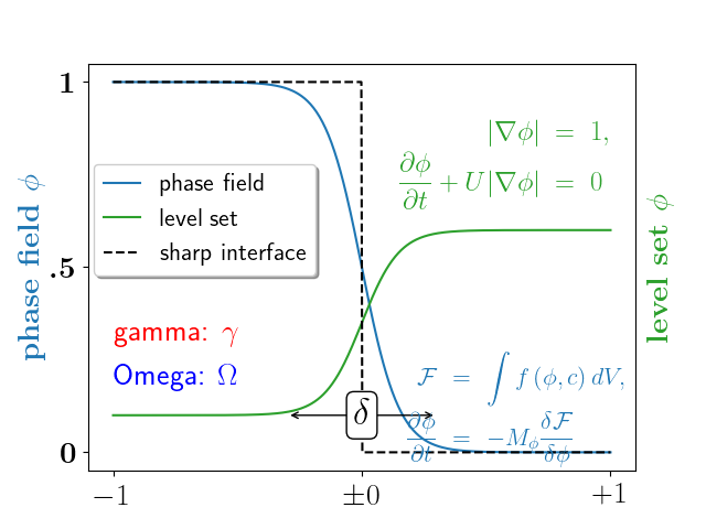
import numpy as npimport matplotlib.pyplot as pltplt.rc('text', usetex=True)# interface tracking profilesN = 500delta = 0.6X = np.linspace(-1, 1, N)plt.plot(X, (1 - np.tanh(4 * X / delta)) / 2, # phase field tanh profilesX, (1.4 + np.tanh(4 * X / delta)) / 4, "C2", # composition profileX, X < 0, 'k--') # sharp interface# legendplt.legend(('phase field', 'level set', 'sharp interface'),shadow=True, loc=(0.01, 0.48), handlelength=1.5, fontsize=16)# the arrowplt.annotate("", xy=(-delta / 2., 0.1), xycoords='data',xytext=(delta / 2., 0.1), textcoords='data',arrowprops=dict(arrowstyle="<->", connectionstyle="arc3"))plt.text(0, 0.1, r'$\delta$',{'color': 'k', 'fontsize': 24, 'ha': 'center', 'va': 'center','bbox': dict(boxstyle="round", fc="w", ec="k", pad=0.2)})# Use tex in labelsplt.xticks((-1, 0, 1), ('$-1$', r'$\pm 0$', '$+1$'), color='k', size=20)# Left Y-axis labels, combine math mode and text modeplt.ylabel(r'\bf{phase field} $\phi$', {'color': 'C0', 'fontsize': 20})plt.yticks((0, 0.5, 1), (r'\bf{0}', r'\bf{.5}', r'\bf{1}'), color='k', size=20)# Right Y-axis labelsplt.text(1.02, 0.5, r"\bf{level set} $\phi$", {'color': 'C2', 'fontsize': 20},horizontalalignment='left',verticalalignment='center',rotation=90,clip_on=False,transform=plt.gca().transAxes)# Use multiline environment inside a `text`.# level set equationseq1 = r"\begin{eqnarray*}" + \r"|\nabla\phi| &=& 1,\\" + \r"\frac{\partial \phi}{\partial t} + U|\nabla \phi| &=& 0 " + \r"\end{eqnarray*}"plt.text(1, 0.9, eq1, {'color': 'C2', 'fontsize': 18}, va="top", ha="right")# phase field equationseq2 = r'\begin{eqnarray*}' + \r'\mathcal{F} &=& \int f\left( \phi, c \right) dV, \\ ' + \r'\frac{ \partial \phi } { \partial t } &=& -M_{ \phi } ' + \r'\frac{ \delta \mathcal{F} } { \delta \phi }' + \r'\end{eqnarray*}'plt.text(0.18, 0.18, eq2, {'color': 'C0', 'fontsize': 16})plt.text(-1, .30, r'gamma: $\gamma$', {'color': 'r', 'fontsize': 20})plt.text(-1, .18, r'Omega: $\Omega$', {'color': 'b', 'fontsize': 20})plt.show()
下载这个示例

若有收获,就点个赞吧
0 人点赞
