等高线图像
等高线,填充等高线和图像绘制的测试组合。 有关等高线标记,另请参见等高线演示示例。
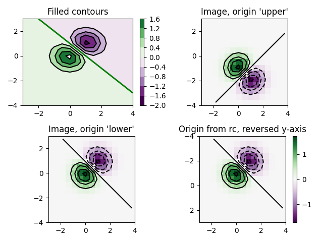
本演示的重点是展示如何在图像上正确展示等高线,以及如何使两者按照需要定向。 特别要注意 “origin”和“extent” 关键字参数在imshow和contour中的用法。
import matplotlib.pyplot as pltimport numpy as npfrom matplotlib import cm# Default delta is large because that makes it fast, and it illustrates# the correct registration between image and contours.delta = 0.5extent = (-3, 4, -4, 3)x = np.arange(-3.0, 4.001, delta)y = np.arange(-4.0, 3.001, delta)X, Y = np.meshgrid(x, y)Z1 = np.exp(-X**2 - Y**2)Z2 = np.exp(-(X - 1)**2 - (Y - 1)**2)Z = (Z1 - Z2) * 2# Boost the upper limit to avoid truncation errors.levels = np.arange(-2.0, 1.601, 0.4)norm = cm.colors.Normalize(vmax=abs(Z).max(), vmin=-abs(Z).max())cmap = cm.PRGnfig, _axs = plt.subplots(nrows=2, ncols=2)fig.subplots_adjust(hspace=0.3)axs = _axs.flatten()cset1 = axs[0].contourf(X, Y, Z, levels, norm=norm,cmap=cm.get_cmap(cmap, len(levels) - 1))# It is not necessary, but for the colormap, we need only the# number of levels minus 1. To avoid discretization error, use# either this number or a large number such as the default (256).# If we want lines as well as filled regions, we need to call# contour separately; don't try to change the edgecolor or edgewidth# of the polygons in the collections returned by contourf.# Use levels output from previous call to guarantee they are the same.cset2 = axs[0].contour(X, Y, Z, cset1.levels, colors='k')# We don't really need dashed contour lines to indicate negative# regions, so let's turn them off.for c in cset2.collections:c.set_linestyle('solid')# It is easier here to make a separate call to contour than# to set up an array of colors and linewidths.# We are making a thick green line as a zero contour.# Specify the zero level as a tuple with only 0 in it.cset3 = axs[0].contour(X, Y, Z, (0,), colors='g', linewidths=2)axs[0].set_title('Filled contours')fig.colorbar(cset1, ax=axs[0])axs[1].imshow(Z, extent=extent, cmap=cmap, norm=norm)axs[1].contour(Z, levels, colors='k', origin='upper', extent=extent)axs[1].set_title("Image, origin 'upper'")axs[2].imshow(Z, origin='lower', extent=extent, cmap=cmap, norm=norm)axs[2].contour(Z, levels, colors='k', origin='lower', extent=extent)axs[2].set_title("Image, origin 'lower'")# We will use the interpolation "nearest" here to show the actual# image pixels.# Note that the contour lines don't extend to the edge of the box.# This is intentional. The Z values are defined at the center of each# image pixel (each color block on the following subplot), so the# domain that is contoured does not extend beyond these pixel centers.im = axs[3].imshow(Z, interpolation='nearest', extent=extent,cmap=cmap, norm=norm)axs[3].contour(Z, levels, colors='k', origin='image', extent=extent)ylim = axs[3].get_ylim()axs[3].set_ylim(ylim[::-1])axs[3].set_title("Origin from rc, reversed y-axis")fig.colorbar(im, ax=axs[3])fig.tight_layout()plt.show()
参考
本例中显示了以下函数、方法和类的使用:
import matplotlibmatplotlib.axes.Axes.contourmatplotlib.pyplot.contourmatplotlib.axes.Axes.imshowmatplotlib.pyplot.imshowmatplotlib.figure.Figure.colorbarmatplotlib.pyplot.colorbarmatplotlib.colors.Normalize
下载这个示例

若有收获,就点个赞吧
0 人点赞
