桑基图类
通过生成三个基本图表来演示Sankey类。
import matplotlib.pyplot as pltfrom matplotlib.sankey import Sankey
示例1 - 主要是默认值
这演示了如何通过隐式调用Sankey.add()方法并将finish()附加到类的调用来创建一个简单的图。
Sankey(flows=[0.25, 0.15, 0.60, -0.20, -0.15, -0.05, -0.50, -0.10],labels=['', '', '', 'First', 'Second', 'Third', 'Fourth', 'Fifth'],orientations=[-1, 1, 0, 1, 1, 1, 0, -1]).finish()plt.title("The default settings produce a diagram like this.")

注意:
示例2
这表明:
fig = plt.figure()ax = fig.add_subplot(1, 1, 1, xticks=[], yticks=[],title="Flow Diagram of a Widget")sankey = Sankey(ax=ax, scale=0.01, offset=0.2, head_angle=180,format='%.0f', unit='%')sankey.add(flows=[25, 0, 60, -10, -20, -5, -15, -10, -40],labels=['', '', '', 'First', 'Second', 'Third', 'Fourth','Fifth', 'Hurray!'],orientations=[-1, 1, 0, 1, 1, 1, -1, -1, 0],pathlengths=[0.25, 0.25, 0.25, 0.25, 0.25, 0.6, 0.25, 0.25,0.25],patchlabel="Widget\nA") # Arguments to matplotlib.patches.PathPatch()diagrams = sankey.finish()diagrams[0].texts[-1].set_color('r')diagrams[0].text.set_fontweight('bold')
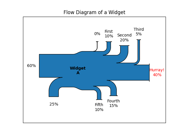
注意:
示例3
这表明:
fig = plt.figure()ax = fig.add_subplot(1, 1, 1, xticks=[], yticks=[], title="Two Systems")flows = [0.25, 0.15, 0.60, -0.10, -0.05, -0.25, -0.15, -0.10, -0.35]sankey = Sankey(ax=ax, unit=None)sankey.add(flows=flows, label='one',orientations=[-1, 1, 0, 1, 1, 1, -1, -1, 0])sankey.add(flows=[-0.25, 0.15, 0.1], label='two',orientations=[-1, -1, -1], prior=0, connect=(0, 0))diagrams = sankey.finish()diagrams[-1].patch.set_hatch('/')plt.legend()
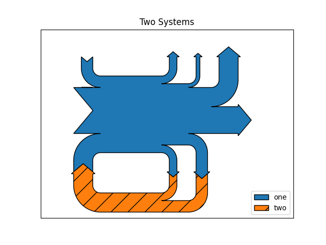
请注意,只指定了一个连接,但系统形成一个电路,因为:(1)路径的长度是合理的,(2)流的方向和顺序是镜像的。
plt.show()
参考
此示例中显示了以下函数,方法,类和模块的使用:
import matplotlibmatplotlib.sankeymatplotlib.sankey.Sankeymatplotlib.sankey.Sankey.addmatplotlib.sankey.Sankey.finish
下载这个示例

若有收获,就点个赞吧
0 人点赞
