使用直方图绘制累积分布
这展示了如何绘制一个累积的、归一化的直方图作为一个步骤函数,以便可视化一个样本的经验累积分布函数(CDF)。文中还给出了理论上的CDF值。
演示了 hist 函数的其他几个选项。也就是说,我们使用 normed 参数来标准化直方图以及 累积 参数的几个不同选项。normed参数采用布尔值。 如果为 True ,则会对箱高进行缩放,使得柱状图的总面积为1。累积的kwarg稍微有些细微差别。与normed一样,您可以将其传递为True或False,但您也可以将其传递-1以反转分布。
由于我们显示了归一化和累积直方图,因此这些曲线实际上是样本的累积分布函数(CDF)。 在工程学中,经验CDF有时被称为“非超越”曲线。 换句话说,您可以查看给定-x值的y值,以使样本的概率和观察值不超过该x值。 例如,x轴上的值225对应于y轴上的约0.85,因此样本中的观察值不超过225的可能性为85%。相反,设置累积为-1,如同已完成 在此示例的最后一个系列中,创建“超出”曲线。
选择不同的箱数和大小会显着影响直方图的形状。Astropy文档有关于如何选择这些参数的重要部分:http://docs.astropy.org/en/stable/visualization/histogram.html
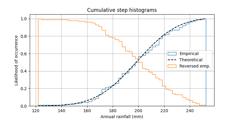
import numpy as npimport matplotlib.pyplot as pltnp.random.seed(19680801)mu = 200sigma = 25n_bins = 50x = np.random.normal(mu, sigma, size=100)fig, ax = plt.subplots(figsize=(8, 4))# plot the cumulative histogramn, bins, patches = ax.hist(x, n_bins, density=True, histtype='step',cumulative=True, label='Empirical')# Add a line showing the expected distribution.y = ((1 / (np.sqrt(2 * np.pi) * sigma)) *np.exp(-0.5 * (1 / sigma * (bins - mu))**2))y = y.cumsum()y /= y[-1]ax.plot(bins, y, 'k--', linewidth=1.5, label='Theoretical')# Overlay a reversed cumulative histogram.ax.hist(x, bins=bins, density=True, histtype='step', cumulative=-1,label='Reversed emp.')# tidy up the figureax.grid(True)ax.legend(loc='right')ax.set_title('Cumulative step histograms')ax.set_xlabel('Annual rainfall (mm)')ax.set_ylabel('Likelihood of occurrence')plt.show()
下载这个示例

若有收获,就点个赞吧
0 人点赞
