着色示例
显示如何制作阴影浮雕图的示例,如Mathematica (http://reference.wolfram.com/mathematica/ref/ReliefPlot.html)或通用映射工具(https://gmt.soest.hawaii.edu/)
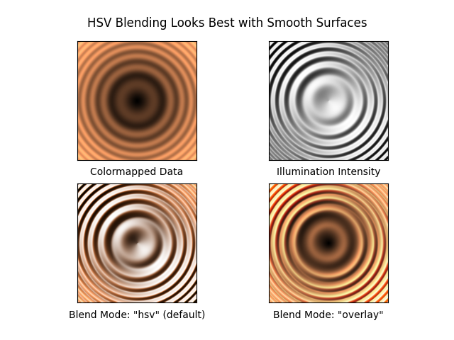
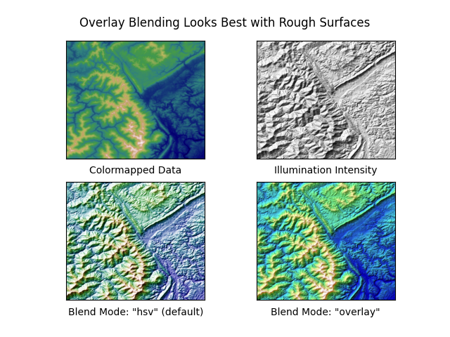
import numpy as npimport matplotlib.pyplot as pltfrom matplotlib.colors import LightSourcefrom matplotlib.cbook import get_sample_datadef main():# Test datax, y = np.mgrid[-5:5:0.05, -5:5:0.05]z = 5 * (np.sqrt(x**2 + y**2) + np.sin(x**2 + y**2))filename = get_sample_data('jacksboro_fault_dem.npz', asfileobj=False)with np.load(filename) as dem:elev = dem['elevation']fig = compare(z, plt.cm.copper)fig.suptitle('HSV Blending Looks Best with Smooth Surfaces', y=0.95)fig = compare(elev, plt.cm.gist_earth, ve=0.05)fig.suptitle('Overlay Blending Looks Best with Rough Surfaces', y=0.95)plt.show()def compare(z, cmap, ve=1):# Create subplots and hide ticksfig, axs = plt.subplots(ncols=2, nrows=2)for ax in axs.flat:ax.set(xticks=[], yticks=[])# Illuminate the scene from the northwestls = LightSource(azdeg=315, altdeg=45)axs[0, 0].imshow(z, cmap=cmap)axs[0, 0].set(xlabel='Colormapped Data')axs[0, 1].imshow(ls.hillshade(z, vert_exag=ve), cmap='gray')axs[0, 1].set(xlabel='Illumination Intensity')rgb = ls.shade(z, cmap=cmap, vert_exag=ve, blend_mode='hsv')axs[1, 0].imshow(rgb)axs[1, 0].set(xlabel='Blend Mode: "hsv" (default)')rgb = ls.shade(z, cmap=cmap, vert_exag=ve, blend_mode='overlay')axs[1, 1].imshow(rgb)axs[1, 1].set(xlabel='Blend Mode: "overlay"')return figif __name__ == '__main__':main()
参考
本例中显示了以下函数、方法和类的使用:
import matplotlibmatplotlib.colors.LightSourcematplotlib.axes.Axes.imshowmatplotlib.pyplot.imshow
下载这个示例

若有收获,就点个赞吧
0 人点赞
