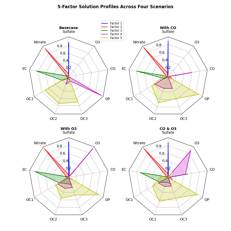
雷达图(又名蜘蛛星图)
此示例创建雷达图表,也称为蜘蛛星图。
虽然此示例允许“圆”或“多边形”的框架,但多边形框架没有合适的网格线(线条是圆形而不是多边形)。 通过将matplotlib.axis中的GRIDLINE_INTERPOLATION_STEPS设置为所需的顶点数,可以获得多边形网格,但多边形的方向不与径向轴对齐。
http://en.wikipedia.org/wiki/Radar_chart
import numpy as npimport matplotlib.pyplot as pltfrom matplotlib.path import Pathfrom matplotlib.spines import Spinefrom matplotlib.projections.polar import PolarAxesfrom matplotlib.projections import register_projectiondef radar_factory(num_vars, frame='circle'):"""Create a radar chart with `num_vars` axes.This function creates a RadarAxes projection and registers it.Parameters----------num_vars : intNumber of variables for radar chart.frame : {'circle' | 'polygon'}Shape of frame surrounding axes."""# calculate evenly-spaced axis anglestheta = np.linspace(0, 2*np.pi, num_vars, endpoint=False)def draw_poly_patch(self):# rotate theta such that the first axis is at the topverts = unit_poly_verts(theta + np.pi / 2)return plt.Polygon(verts, closed=True, edgecolor='k')def draw_circle_patch(self):# unit circle centered on (0.5, 0.5)return plt.Circle((0.5, 0.5), 0.5)patch_dict = {'polygon': draw_poly_patch, 'circle': draw_circle_patch}if frame not in patch_dict:raise ValueError('unknown value for `frame`: %s' % frame)class RadarAxes(PolarAxes):name = 'radar'# use 1 line segment to connect specified pointsRESOLUTION = 1# define draw_frame methoddraw_patch = patch_dict[frame]def __init__(self, *args, **kwargs):super().__init__(*args, **kwargs)# rotate plot such that the first axis is at the topself.set_theta_zero_location('N')def fill(self, *args, closed=True, **kwargs):"""Override fill so that line is closed by default"""return super().fill(closed=closed, *args, **kwargs)def plot(self, *args, **kwargs):"""Override plot so that line is closed by default"""lines = super().plot(*args, **kwargs)for line in lines:self._close_line(line)def _close_line(self, line):x, y = line.get_data()# FIXME: markers at x[0], y[0] get doubled-upif x[0] != x[-1]:x = np.concatenate((x, [x[0]]))y = np.concatenate((y, [y[0]]))line.set_data(x, y)def set_varlabels(self, labels):self.set_thetagrids(np.degrees(theta), labels)def _gen_axes_patch(self):return self.draw_patch()def _gen_axes_spines(self):if frame == 'circle':return super()._gen_axes_spines()# The following is a hack to get the spines (i.e. the axes frame)# to draw correctly for a polygon frame.# spine_type must be 'left', 'right', 'top', 'bottom', or `circle`.spine_type = 'circle'verts = unit_poly_verts(theta + np.pi / 2)# close off polygon by repeating first vertexverts.append(verts[0])path = Path(verts)spine = Spine(self, spine_type, path)spine.set_transform(self.transAxes)return {'polar': spine}register_projection(RadarAxes)return thetadef unit_poly_verts(theta):"""Return vertices of polygon for subplot axes.This polygon is circumscribed by a unit circle centered at (0.5, 0.5)"""x0, y0, r = [0.5] * 3verts = [(r*np.cos(t) + x0, r*np.sin(t) + y0) for t in theta]return vertsdef example_data():# The following data is from the Denver Aerosol Sources and Health study.# See doi:10.1016/j.atmosenv.2008.12.017## The data are pollution source profile estimates for five modeled# pollution sources (e.g., cars, wood-burning, etc) that emit 7-9 chemical# species. The radar charts are experimented with here to see if we can# nicely visualize how the modeled source profiles change across four# scenarios:# 1) No gas-phase species present, just seven particulate counts on# Sulfate# Nitrate# Elemental Carbon (EC)# Organic Carbon fraction 1 (OC)# Organic Carbon fraction 2 (OC2)# Organic Carbon fraction 3 (OC3)# Pyrolized Organic Carbon (OP)# 2)Inclusion of gas-phase specie carbon monoxide (CO)# 3)Inclusion of gas-phase specie ozone (O3).# 4)Inclusion of both gas-phase species is present...data = [['Sulfate', 'Nitrate', 'EC', 'OC1', 'OC2', 'OC3', 'OP', 'CO', 'O3'],('Basecase', [[0.88, 0.01, 0.03, 0.03, 0.00, 0.06, 0.01, 0.00, 0.00],[0.07, 0.95, 0.04, 0.05, 0.00, 0.02, 0.01, 0.00, 0.00],[0.01, 0.02, 0.85, 0.19, 0.05, 0.10, 0.00, 0.00, 0.00],[0.02, 0.01, 0.07, 0.01, 0.21, 0.12, 0.98, 0.00, 0.00],[0.01, 0.01, 0.02, 0.71, 0.74, 0.70, 0.00, 0.00, 0.00]]),('With CO', [[0.88, 0.02, 0.02, 0.02, 0.00, 0.05, 0.00, 0.05, 0.00],[0.08, 0.94, 0.04, 0.02, 0.00, 0.01, 0.12, 0.04, 0.00],[0.01, 0.01, 0.79, 0.10, 0.00, 0.05, 0.00, 0.31, 0.00],[0.00, 0.02, 0.03, 0.38, 0.31, 0.31, 0.00, 0.59, 0.00],[0.02, 0.02, 0.11, 0.47, 0.69, 0.58, 0.88, 0.00, 0.00]]),('With O3', [[0.89, 0.01, 0.07, 0.00, 0.00, 0.05, 0.00, 0.00, 0.03],[0.07, 0.95, 0.05, 0.04, 0.00, 0.02, 0.12, 0.00, 0.00],[0.01, 0.02, 0.86, 0.27, 0.16, 0.19, 0.00, 0.00, 0.00],[0.01, 0.03, 0.00, 0.32, 0.29, 0.27, 0.00, 0.00, 0.95],[0.02, 0.00, 0.03, 0.37, 0.56, 0.47, 0.87, 0.00, 0.00]]),('CO & O3', [[0.87, 0.01, 0.08, 0.00, 0.00, 0.04, 0.00, 0.00, 0.01],[0.09, 0.95, 0.02, 0.03, 0.00, 0.01, 0.13, 0.06, 0.00],[0.01, 0.02, 0.71, 0.24, 0.13, 0.16, 0.00, 0.50, 0.00],[0.01, 0.03, 0.00, 0.28, 0.24, 0.23, 0.00, 0.44, 0.88],[0.02, 0.00, 0.18, 0.45, 0.64, 0.55, 0.86, 0.00, 0.16]])]return dataif __name__ == '__main__':N = 9theta = radar_factory(N, frame='polygon')data = example_data()spoke_labels = data.pop(0)fig, axes = plt.subplots(figsize=(9, 9), nrows=2, ncols=2,subplot_kw=dict(projection='radar'))fig.subplots_adjust(wspace=0.25, hspace=0.20, top=0.85, bottom=0.05)colors = ['b', 'r', 'g', 'm', 'y']# Plot the four cases from the example data on separate axesfor ax, (title, case_data) in zip(axes.flatten(), data):ax.set_rgrids([0.2, 0.4, 0.6, 0.8])ax.set_title(title, weight='bold', size='medium', position=(0.5, 1.1),horizontalalignment='center', verticalalignment='center')for d, color in zip(case_data, colors):ax.plot(theta, d, color=color)ax.fill(theta, d, facecolor=color, alpha=0.25)ax.set_varlabels(spoke_labels)# add legend relative to top-left plotax = axes[0, 0]labels = ('Factor 1', 'Factor 2', 'Factor 3', 'Factor 4', 'Factor 5')legend = ax.legend(labels, loc=(0.9, .95),labelspacing=0.1, fontsize='small')fig.text(0.5, 0.965, '5-Factor Solution Profiles Across Four Scenarios',horizontalalignment='center', color='black', weight='bold',size='large')plt.show()
参考
此示例中显示了以下函数,方法,类和模块的使用:
import matplotlibmatplotlib.pathmatplotlib.path.Pathmatplotlib.spinesmatplotlib.spines.Spinematplotlib.projectionsmatplotlib.projections.polarmatplotlib.projections.polar.PolarAxesmatplotlib.projections.register_projection
下载这个示例

若有收获,就点个赞吧
0 人点赞
