演示Curvelinear网格
自定义网格和记号行。
此示例演示如何通过在网格上应用转换,使用GridHelperCurve线性来定义自定义网格和注释行。这可以用作第二个打印上的演示,用于在矩形框中创建极轴投影。
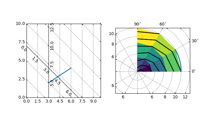
import numpy as npimport matplotlib.pyplot as pltimport matplotlib.cbook as cbookfrom mpl_toolkits.axisartist import Subplotfrom mpl_toolkits.axisartist import SubplotHost, \ParasiteAxesAuxTransfrom mpl_toolkits.axisartist.grid_helper_curvelinear import \GridHelperCurveLineardef curvelinear_test1(fig):"""grid for custom transform."""def tr(x, y):x, y = np.asarray(x), np.asarray(y)return x, y - xdef inv_tr(x, y):x, y = np.asarray(x), np.asarray(y)return x, y + xgrid_helper = GridHelperCurveLinear((tr, inv_tr))ax1 = Subplot(fig, 1, 2, 1, grid_helper=grid_helper)# ax1 will have a ticks and gridlines defined by the given# transform (+ transData of the Axes). Note that the transform of# the Axes itself (i.e., transData) is not affected by the given# transform.fig.add_subplot(ax1)xx, yy = tr([3, 6], [5.0, 10.])ax1.plot(xx, yy, linewidth=2.0)ax1.set_aspect(1.)ax1.set_xlim(0, 10.)ax1.set_ylim(0, 10.)ax1.axis["t"] = ax1.new_floating_axis(0, 3.)ax1.axis["t2"] = ax1.new_floating_axis(1, 7.)ax1.grid(True, zorder=0)import mpl_toolkits.axisartist.angle_helper as angle_helperfrom matplotlib.projections import PolarAxesfrom matplotlib.transforms import Affine2Ddef curvelinear_test2(fig):"""polar projection, but in a rectangular box."""# PolarAxes.PolarTransform takes radian. However, we want our coordinate# system in degreetr = Affine2D().scale(np.pi/180., 1.) + PolarAxes.PolarTransform()# polar projection, which involves cycle, and also has limits in# its coordinates, needs a special method to find the extremes# (min, max of the coordinate within the view).# 20, 20 : number of sampling points along x, y directionextreme_finder = angle_helper.ExtremeFinderCycle(20, 20,lon_cycle=360,lat_cycle=None,lon_minmax=None,lat_minmax=(0, np.inf),)grid_locator1 = angle_helper.LocatorDMS(12)# Find a grid values appropriate for the coordinate (degree,# minute, second).tick_formatter1 = angle_helper.FormatterDMS()# And also uses an appropriate formatter. Note that,the# acceptable Locator and Formatter class is a bit different than# that of mpl's, and you cannot directly use mpl's Locator and# Formatter here (but may be possible in the future).grid_helper = GridHelperCurveLinear(tr,extreme_finder=extreme_finder,grid_locator1=grid_locator1,tick_formatter1=tick_formatter1)ax1 = SubplotHost(fig, 1, 2, 2, grid_helper=grid_helper)# make ticklabels of right and top axis visible.ax1.axis["right"].major_ticklabels.set_visible(True)ax1.axis["top"].major_ticklabels.set_visible(True)# let right axis shows ticklabels for 1st coordinate (angle)ax1.axis["right"].get_helper().nth_coord_ticks = 0# let bottom axis shows ticklabels for 2nd coordinate (radius)ax1.axis["bottom"].get_helper().nth_coord_ticks = 1fig.add_subplot(ax1)# A parasite axes with given transformax2 = ParasiteAxesAuxTrans(ax1, tr, "equal")# note that ax2.transData == tr + ax1.transData# Anything you draw in ax2 will match the ticks and grids of ax1.ax1.parasites.append(ax2)intp = cbook.simple_linear_interpolationax2.plot(intp(np.array([0, 30]), 50),intp(np.array([10., 10.]), 50),linewidth=2.0)ax1.set_aspect(1.)ax1.set_xlim(-5, 12)ax1.set_ylim(-5, 10)ax1.grid(True, zorder=0)if 1:fig = plt.figure(1, figsize=(7, 4))fig.clf()curvelinear_test1(fig)curvelinear_test2(fig)plt.show()
下载这个示例

若有收获,就点个赞吧
0 人点赞
