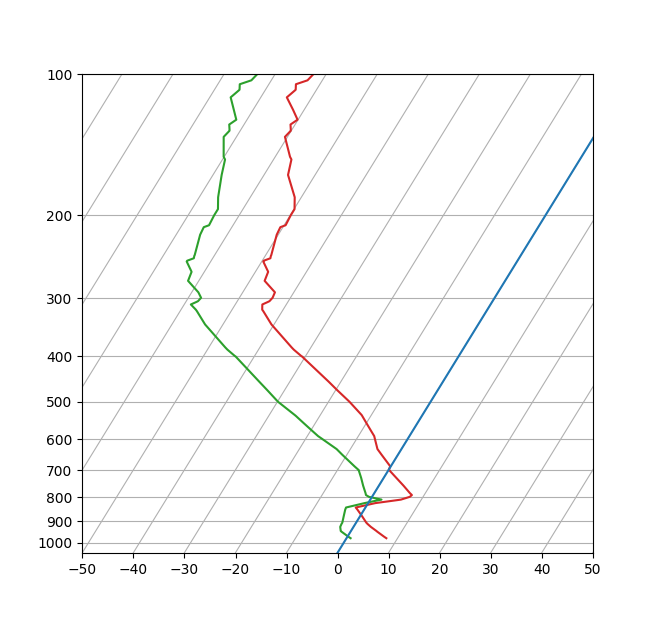
SkewT-logP图:使用变换和自定义投影
这可以作为matplotlib变换和自定义投影API的强化练习。 这个例子产生了一个所谓的SkewT-logP图,它是气象学中用于显示温度垂直剖面的常见图。 就matplotlib而言,复杂性来自于X轴和Y轴不正交。 这是通过在基本Axes变换中包含一个偏斜分量来处理的。 处理上下X轴具有不同数据范围的事实带来了额外的复杂性,这需要一系列用于刻度,棘轮和轴的自定义类来处理这一问题。
from matplotlib.axes import Axesimport matplotlib.transforms as transformsimport matplotlib.axis as maxisimport matplotlib.spines as mspinesfrom matplotlib.projections import register_projection# The sole purpose of this class is to look at the upper, lower, or total# interval as appropriate and see what parts of the tick to draw, if any.class SkewXTick(maxis.XTick):def update_position(self, loc):# This ensures that the new value of the location is set before# any other updates take placeself._loc = locsuper().update_position(loc)def _has_default_loc(self):return self.get_loc() is Nonedef _need_lower(self):return (self._has_default_loc() ortransforms.interval_contains(self.axes.lower_xlim,self.get_loc()))def _need_upper(self):return (self._has_default_loc() ortransforms.interval_contains(self.axes.upper_xlim,self.get_loc()))@propertydef gridOn(self):return (self._gridOn and (self._has_default_loc() ortransforms.interval_contains(self.get_view_interval(),self.get_loc())))@gridOn.setterdef gridOn(self, value):self._gridOn = value@propertydef tick1On(self):return self._tick1On and self._need_lower()@tick1On.setterdef tick1On(self, value):self._tick1On = value@propertydef label1On(self):return self._label1On and self._need_lower()@label1On.setterdef label1On(self, value):self._label1On = value@propertydef tick2On(self):return self._tick2On and self._need_upper()@tick2On.setterdef tick2On(self, value):self._tick2On = value@propertydef label2On(self):return self._label2On and self._need_upper()@label2On.setterdef label2On(self, value):self._label2On = valuedef get_view_interval(self):return self.axes.xaxis.get_view_interval()# This class exists to provide two separate sets of intervals to the tick,# as well as create instances of the custom tickclass SkewXAxis(maxis.XAxis):def _get_tick(self, major):return SkewXTick(self.axes, None, '', major=major)def get_view_interval(self):return self.axes.upper_xlim[0], self.axes.lower_xlim[1]# This class exists to calculate the separate data range of the# upper X-axis and draw the spine there. It also provides this range# to the X-axis artist for ticking and gridlinesclass SkewSpine(mspines.Spine):def _adjust_location(self):pts = self._path.verticesif self.spine_type == 'top':pts[:, 0] = self.axes.upper_xlimelse:pts[:, 0] = self.axes.lower_xlim# This class handles registration of the skew-xaxes as a projection as well# as setting up the appropriate transformations. It also overrides standard# spines and axes instances as appropriate.class SkewXAxes(Axes):# The projection must specify a name. This will be used be the# user to select the projection, i.e. ``subplot(111,# projection='skewx')``.name = 'skewx'def _init_axis(self):# Taken from Axes and modified to use our modified X-axisself.xaxis = SkewXAxis(self)self.spines['top'].register_axis(self.xaxis)self.spines['bottom'].register_axis(self.xaxis)self.yaxis = maxis.YAxis(self)self.spines['left'].register_axis(self.yaxis)self.spines['right'].register_axis(self.yaxis)def _gen_axes_spines(self):spines = {'top': SkewSpine.linear_spine(self, 'top'),'bottom': mspines.Spine.linear_spine(self, 'bottom'),'left': mspines.Spine.linear_spine(self, 'left'),'right': mspines.Spine.linear_spine(self, 'right')}return spinesdef _set_lim_and_transforms(self):"""This is called once when the plot is created to set up all thetransforms for the data, text and grids."""rot = 30# Get the standard transform setup from the Axes base classAxes._set_lim_and_transforms(self)# Need to put the skew in the middle, after the scale and limits,# but before the transAxes. This way, the skew is done in Axes# coordinates thus performing the transform around the proper origin# We keep the pre-transAxes transform around for other users, like the# spines for finding boundsself.transDataToAxes = self.transScale + \self.transLimits + transforms.Affine2D().skew_deg(rot, 0)# Create the full transform from Data to Pixelsself.transData = self.transDataToAxes + self.transAxes# Blended transforms like this need to have the skewing applied using# both axes, in axes coords like before.self._xaxis_transform = (transforms.blended_transform_factory(self.transScale + self.transLimits,transforms.IdentityTransform()) +transforms.Affine2D().skew_deg(rot, 0)) + self.transAxes@propertydef lower_xlim(self):return self.axes.viewLim.intervalx@propertydef upper_xlim(self):pts = [[0., 1.], [1., 1.]]return self.transDataToAxes.inverted().transform(pts)[:, 0]# Now register the projection with matplotlib so the user can select# it.register_projection(SkewXAxes)if __name__ == '__main__':# Now make a simple example using the custom projection.from io import StringIOfrom matplotlib.ticker import (MultipleLocator, NullFormatter,ScalarFormatter)import matplotlib.pyplot as pltimport numpy as np# Some examples datadata_txt = '''978.0 345 7.8 0.8 61 4.16 325 14 282.7 294.6 283.4971.0 404 7.2 0.2 61 4.01 327 17 282.7 294.2 283.4946.7 610 5.2 -1.8 61 3.56 335 26 282.8 293.0 283.4944.0 634 5.0 -2.0 61 3.51 336 27 282.8 292.9 283.4925.0 798 3.4 -2.6 65 3.43 340 32 282.8 292.7 283.4911.8 914 2.4 -2.7 69 3.46 345 37 282.9 292.9 283.5906.0 966 2.0 -2.7 71 3.47 348 39 283.0 293.0 283.6877.9 1219 0.4 -3.2 77 3.46 0 48 283.9 293.9 284.5850.0 1478 -1.3 -3.7 84 3.44 0 47 284.8 294.8 285.4841.0 1563 -1.9 -3.8 87 3.45 358 45 285.0 295.0 285.6823.0 1736 1.4 -0.7 86 4.44 353 42 290.3 303.3 291.0813.6 1829 4.5 1.2 80 5.17 350 40 294.5 309.8 295.4809.0 1875 6.0 2.2 77 5.57 347 39 296.6 313.2 297.6798.0 1988 7.4 -0.6 57 4.61 340 35 299.2 313.3 300.1791.0 2061 7.6 -1.4 53 4.39 335 33 300.2 313.6 301.0783.9 2134 7.0 -1.7 54 4.32 330 31 300.4 313.6 301.2755.1 2438 4.8 -3.1 57 4.06 300 24 301.2 313.7 301.9727.3 2743 2.5 -4.4 60 3.81 285 29 301.9 313.8 302.6700.5 3048 0.2 -5.8 64 3.57 275 31 302.7 313.8 303.3700.0 3054 0.2 -5.8 64 3.56 280 31 302.7 313.8 303.3698.0 3077 0.0 -6.0 64 3.52 280 31 302.7 313.7 303.4687.0 3204 -0.1 -7.1 59 3.28 281 31 304.0 314.3 304.6648.9 3658 -3.2 -10.9 55 2.59 285 30 305.5 313.8 305.9631.0 3881 -4.7 -12.7 54 2.29 289 33 306.2 313.6 306.6600.7 4267 -6.4 -16.7 44 1.73 295 39 308.6 314.3 308.9592.0 4381 -6.9 -17.9 41 1.59 297 41 309.3 314.6 309.6577.6 4572 -8.1 -19.6 39 1.41 300 44 310.1 314.9 310.3555.3 4877 -10.0 -22.3 36 1.16 295 39 311.3 315.3 311.5536.0 5151 -11.7 -24.7 33 0.97 304 39 312.4 315.8 312.6533.8 5182 -11.9 -25.0 33 0.95 305 39 312.5 315.8 312.7500.0 5680 -15.9 -29.9 29 0.64 290 44 313.6 315.9 313.7472.3 6096 -19.7 -33.4 28 0.49 285 46 314.1 315.8 314.1453.0 6401 -22.4 -36.0 28 0.39 300 50 314.4 315.8 314.4400.0 7310 -30.7 -43.7 27 0.20 285 44 315.0 315.8 315.0399.7 7315 -30.8 -43.8 27 0.20 285 44 315.0 315.8 315.0387.0 7543 -33.1 -46.1 26 0.16 281 47 314.9 315.5 314.9382.7 7620 -33.8 -46.8 26 0.15 280 48 315.0 315.6 315.0342.0 8398 -40.5 -53.5 23 0.08 293 52 316.1 316.4 316.1320.4 8839 -43.7 -56.7 22 0.06 300 54 317.6 317.8 317.6318.0 8890 -44.1 -57.1 22 0.05 301 55 317.8 318.0 317.8310.0 9060 -44.7 -58.7 19 0.04 304 61 319.2 319.4 319.2306.1 9144 -43.9 -57.9 20 0.05 305 63 321.5 321.7 321.5305.0 9169 -43.7 -57.7 20 0.05 303 63 322.1 322.4 322.1300.0 9280 -43.5 -57.5 20 0.05 295 64 323.9 324.2 323.9292.0 9462 -43.7 -58.7 17 0.05 293 67 326.2 326.4 326.2276.0 9838 -47.1 -62.1 16 0.03 290 74 326.6 326.7 326.6264.0 10132 -47.5 -62.5 16 0.03 288 79 330.1 330.3 330.1251.0 10464 -49.7 -64.7 16 0.03 285 85 331.7 331.8 331.7250.0 10490 -49.7 -64.7 16 0.03 285 85 332.1 332.2 332.1247.0 10569 -48.7 -63.7 16 0.03 283 88 334.7 334.8 334.7244.0 10649 -48.9 -63.9 16 0.03 280 91 335.6 335.7 335.6243.3 10668 -48.9 -63.9 16 0.03 280 91 335.8 335.9 335.8220.0 11327 -50.3 -65.3 15 0.03 280 85 343.5 343.6 343.5212.0 11569 -50.5 -65.5 15 0.03 280 83 346.8 346.9 346.8210.0 11631 -49.7 -64.7 16 0.03 280 83 349.0 349.1 349.0200.0 11950 -49.9 -64.9 15 0.03 280 80 353.6 353.7 353.6194.0 12149 -49.9 -64.9 15 0.03 279 78 356.7 356.8 356.7183.0 12529 -51.3 -66.3 15 0.03 278 75 360.4 360.5 360.4164.0 13233 -55.3 -68.3 18 0.02 277 69 365.2 365.3 365.2152.0 13716 -56.5 -69.5 18 0.02 275 65 371.1 371.2 371.1150.0 13800 -57.1 -70.1 18 0.02 275 64 371.5 371.6 371.5136.0 14414 -60.5 -72.5 19 0.02 268 54 376.0 376.1 376.0132.0 14600 -60.1 -72.1 19 0.02 265 51 380.0 380.1 380.0131.4 14630 -60.2 -72.2 19 0.02 265 51 380.3 380.4 380.3128.0 14792 -60.9 -72.9 19 0.02 266 50 381.9 382.0 381.9125.0 14939 -60.1 -72.1 19 0.02 268 49 385.9 386.0 385.9119.0 15240 -62.2 -73.8 20 0.01 270 48 387.4 387.5 387.4112.0 15616 -64.9 -75.9 21 0.01 265 53 389.3 389.3 389.3108.0 15838 -64.1 -75.1 21 0.01 265 58 394.8 394.9 394.8107.8 15850 -64.1 -75.1 21 0.01 265 58 395.0 395.1 395.0105.0 16010 -64.7 -75.7 21 0.01 272 50 396.9 396.9 396.9103.0 16128 -62.9 -73.9 21 0.02 277 45 402.5 402.6 402.5100.0 16310 -62.5 -73.5 21 0.02 285 36 406.7 406.8 406.7'''# Parse the datasound_data = StringIO(data_txt)p, h, T, Td = np.loadtxt(sound_data, usecols=range(0, 4), unpack=True)# Create a new figure. The dimensions here give a good aspect ratiofig = plt.figure(figsize=(6.5875, 6.2125))ax = fig.add_subplot(111, projection='skewx')plt.grid(True)# Plot the data using normal plotting functions, in this case using# log scaling in Y, as dictated by the typical meteorological plotax.semilogy(T, p, color='C3')ax.semilogy(Td, p, color='C2')# An example of a slanted line at constant Xl = ax.axvline(0, color='C0')# Disables the log-formatting that comes with semilogyax.yaxis.set_major_formatter(ScalarFormatter())ax.yaxis.set_minor_formatter(NullFormatter())ax.set_yticks(np.linspace(100, 1000, 10))ax.set_ylim(1050, 100)ax.xaxis.set_major_locator(MultipleLocator(10))ax.set_xlim(-50, 50)plt.show()
参考
此示例中显示了以下函数,方法,类和模块的使用:
import matplotlibmatplotlib.transformsmatplotlib.spinesmatplotlib.spines.Spinematplotlib.spines.Spine.register_axismatplotlib.projectionsmatplotlib.projections.register_projection
下载这个示例

若有收获,就点个赞吧
0 人点赞
