数学文本例子
Matplotlib的数学渲染引擎的选定功能。
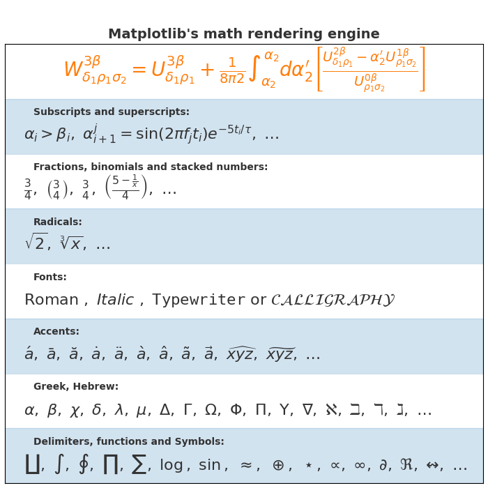
Out:
0 $W^{3\beta}_{\delta_1 \rho_1 \sigma_2} = U^{3\beta}_{\delta_1 \rho_1} + \frac{1}{8 \pi 2} \int^{\alpha_2}_{\alpha_2} d \alpha^\prime_2 \left[\frac{ U^{2\beta}_{\delta_1 \rho_1} - \alpha^\prime_2U^{1\beta}_{\rho_1 \sigma_2} }{U^{0\beta}_{\rho_1 \sigma_2}}\right]$1 $\alpha_i > \beta_i,\ \alpha_{i+1}^j = {\rm sin}(2\pi f_j t_i) e^{-5 t_i/\tau},\ \ldots$2 $\frac{3}{4},\ \binom{3}{4},\ \stackrel{3}{4},\ \left(\frac{5 - \frac{1}{x}}{4}\right),\ \ldots$3 $\sqrt{2},\ \sqrt[3]{x},\ \ldots$4 $\mathrm{Roman}\ , \ \mathit{Italic}\ , \ \mathtt{Typewriter} \ \mathrm{or}\ \mathcal{CALLIGRAPHY}$5 $\acute a,\ \bar a,\ \breve a,\ \dot a,\ \ddot a, \ \grave a, \ \hat a,\ \tilde a,\ \vec a,\ \widehat{xyz},\ \widetilde{xyz},\ \ldots$6 $\alpha,\ \beta,\ \chi,\ \delta,\ \lambda,\ \mu,\ \Delta,\ \Gamma,\ \Omega,\ \Phi,\ \Pi,\ \Upsilon,\ \nabla,\ \aleph,\ \beth,\ \daleth,\ \gimel,\ \ldots$7 $\coprod,\ \int,\ \oint,\ \prod,\ \sum,\ \log,\ \sin,\ \approx,\ \oplus,\ \star,\ \varpropto,\ \infty,\ \partial,\ \Re,\ \leftrightsquigarrow, \ \ldots$
import matplotlib.pyplot as pltimport subprocessimport sysimport re# Selection of features following "Writing mathematical expressions" tutorialmathtext_titles = {0: "Header demo",1: "Subscripts and superscripts",2: "Fractions, binomials and stacked numbers",3: "Radicals",4: "Fonts",5: "Accents",6: "Greek, Hebrew",7: "Delimiters, functions and Symbols"}n_lines = len(mathtext_titles)# Randomly picked examplesmathext_demos = {0: r"$W^{3\beta}_{\delta_1 \rho_1 \sigma_2} = "r"U^{3\beta}_{\delta_1 \rho_1} + \frac{1}{8 \pi 2} "r"\int^{\alpha_2}_{\alpha_2} d \alpha^\prime_2 \left[\frac{ "r"U^{2\beta}_{\delta_1 \rho_1} - \alpha^\prime_2U^{1\beta}_"r"{\rho_1 \sigma_2} }{U^{0\beta}_{\rho_1 \sigma_2}}\right]$",1: r"$\alpha_i > \beta_i,\ "r"\alpha_{i+1}^j = {\rm sin}(2\pi f_j t_i) e^{-5 t_i/\tau},\ "r"\ldots$",2: r"$\frac{3}{4},\ \binom{3}{4},\ \stackrel{3}{4},\ "r"\left(\frac{5 - \frac{1}{x}}{4}\right),\ \ldots$",3: r"$\sqrt{2},\ \sqrt[3]{x},\ \ldots$",4: r"$\mathrm{Roman}\ , \ \mathit{Italic}\ , \ \mathtt{Typewriter} \ "r"\mathrm{or}\ \mathcal{CALLIGRAPHY}$",5: r"$\acute a,\ \bar a,\ \breve a,\ \dot a,\ \ddot a, \ \grave a, \ "r"\hat a,\ \tilde a,\ \vec a,\ \widehat{xyz},\ \widetilde{xyz},\ "r"\ldots$",6: r"$\alpha,\ \beta,\ \chi,\ \delta,\ \lambda,\ \mu,\ "r"\Delta,\ \Gamma,\ \Omega,\ \Phi,\ \Pi,\ \Upsilon,\ \nabla,\ "r"\aleph,\ \beth,\ \daleth,\ \gimel,\ \ldots$",7: r"$\coprod,\ \int,\ \oint,\ \prod,\ \sum,\ "r"\log,\ \sin,\ \approx,\ \oplus,\ \star,\ \varpropto,\ "r"\infty,\ \partial,\ \Re,\ \leftrightsquigarrow, \ \ldots$"}def doall():# Colors used in mpl online documentation.mpl_blue_rvb = (191. / 255., 209. / 256., 212. / 255.)mpl_orange_rvb = (202. / 255., 121. / 256., 0. / 255.)mpl_grey_rvb = (51. / 255., 51. / 255., 51. / 255.)# Creating figure and axis.plt.figure(figsize=(6, 7))plt.axes([0.01, 0.01, 0.98, 0.90], facecolor="white", frameon=True)plt.gca().set_xlim(0., 1.)plt.gca().set_ylim(0., 1.)plt.gca().set_title("Matplotlib's math rendering engine",color=mpl_grey_rvb, fontsize=14, weight='bold')plt.gca().set_xticklabels("", visible=False)plt.gca().set_yticklabels("", visible=False)# Gap between lines in axes coordsline_axesfrac = (1. / (n_lines))# Plotting header demonstration formulafull_demo = mathext_demos[0]plt.annotate(full_demo,xy=(0.5, 1. - 0.59 * line_axesfrac),xycoords='data', color=mpl_orange_rvb, ha='center',fontsize=20)# Plotting features demonstration formulaefor i_line in range(1, n_lines):baseline = 1 - (i_line) * line_axesfracbaseline_next = baseline - line_axesfractitle = mathtext_titles[i_line] + ":"fill_color = ['white', mpl_blue_rvb][i_line % 2]plt.fill_between([0., 1.], [baseline, baseline],[baseline_next, baseline_next],color=fill_color, alpha=0.5)plt.annotate(title,xy=(0.07, baseline - 0.3 * line_axesfrac),xycoords='data', color=mpl_grey_rvb, weight='bold')demo = mathext_demos[i_line]plt.annotate(demo,xy=(0.05, baseline - 0.75 * line_axesfrac),xycoords='data', color=mpl_grey_rvb,fontsize=16)for i in range(n_lines):s = mathext_demos[i]print(i, s)plt.show()if '--latex' in sys.argv:# Run: python mathtext_examples.py --latex# Need amsmath and amssymb packages.fd = open("mathtext_examples.ltx", "w")fd.write("\\documentclass{article}\n")fd.write("\\usepackage{amsmath, amssymb}\n")fd.write("\\begin{document}\n")fd.write("\\begin{enumerate}\n")for i in range(n_lines):s = mathext_demos[i]s = re.sub(r"(?<!\\)\$", "$$", s)fd.write("\\item %s\n" % s)fd.write("\\end{enumerate}\n")fd.write("\\end{document}\n")fd.close()subprocess.call(["pdflatex", "mathtext_examples.ltx"])else:doall()
下载这个示例

若有收获,就点个赞吧
0 人点赞
