左心室靶心
该示例演示了如何为美国心脏协会(AHA)推荐的左心室创建17段模型。
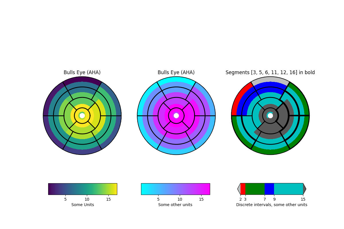
import numpy as npimport matplotlib as mplimport matplotlib.pyplot as pltdef bullseye_plot(ax, data, segBold=None, cmap=None, norm=None):"""Bullseye representation for the left ventricle.Parameters----------ax : axesdata : list of int and floatThe intensity values for each of the 17 segmentssegBold: list of int, optionalA list with the segments to highlightcmap : ColorMap or None, optionalOptional argument to set the desired colormapnorm : Normalize or None, optionalOptional argument to normalize data into the [0.0, 1.0] rangeNotes-----This function create the 17 segment model for the left ventricle accordingto the American Heart Association (AHA) [1]_References----------.. [1] M. D. Cerqueira, N. J. Weissman, V. Dilsizian, A. K. Jacobs,S. Kaul, W. K. Laskey, D. J. Pennell, J. A. Rumberger, T. Ryan,and M. S. Verani, "Standardized myocardial segmentation andnomenclature for tomographic imaging of the heart",Circulation, vol. 105, no. 4, pp. 539-542, 2002."""if segBold is None:segBold = []linewidth = 2data = np.array(data).ravel()if cmap is None:cmap = plt.cm.viridisif norm is None:norm = mpl.colors.Normalize(vmin=data.min(), vmax=data.max())theta = np.linspace(0, 2 * np.pi, 768)r = np.linspace(0.2, 1, 4)# Create the bound for the segment 17for i in range(r.shape[0]):ax.plot(theta, np.repeat(r[i], theta.shape), '-k', lw=linewidth)# Create the bounds for the segments 1-12for i in range(6):theta_i = np.deg2rad(i * 60)ax.plot([theta_i, theta_i], [r[1], 1], '-k', lw=linewidth)# Create the bounds for the segments 13-16for i in range(4):theta_i = np.deg2rad(i * 90 - 45)ax.plot([theta_i, theta_i], [r[0], r[1]], '-k', lw=linewidth)# Fill the segments 1-6r0 = r[2:4]r0 = np.repeat(r0[:, np.newaxis], 128, axis=1).Tfor i in range(6):# First segment start at 60 degreestheta0 = theta[i * 128:i * 128 + 128] + np.deg2rad(60)theta0 = np.repeat(theta0[:, np.newaxis], 2, axis=1)z = np.ones((128, 2)) * data[i]ax.pcolormesh(theta0, r0, z, cmap=cmap, norm=norm)if i + 1 in segBold:ax.plot(theta0, r0, '-k', lw=linewidth + 2)ax.plot(theta0[0], [r[2], r[3]], '-k', lw=linewidth + 1)ax.plot(theta0[-1], [r[2], r[3]], '-k', lw=linewidth + 1)# Fill the segments 7-12r0 = r[1:3]r0 = np.repeat(r0[:, np.newaxis], 128, axis=1).Tfor i in range(6):# First segment start at 60 degreestheta0 = theta[i * 128:i * 128 + 128] + np.deg2rad(60)theta0 = np.repeat(theta0[:, np.newaxis], 2, axis=1)z = np.ones((128, 2)) * data[i + 6]ax.pcolormesh(theta0, r0, z, cmap=cmap, norm=norm)if i + 7 in segBold:ax.plot(theta0, r0, '-k', lw=linewidth + 2)ax.plot(theta0[0], [r[1], r[2]], '-k', lw=linewidth + 1)ax.plot(theta0[-1], [r[1], r[2]], '-k', lw=linewidth + 1)# Fill the segments 13-16r0 = r[0:2]r0 = np.repeat(r0[:, np.newaxis], 192, axis=1).Tfor i in range(4):# First segment start at 45 degreestheta0 = theta[i * 192:i * 192 + 192] + np.deg2rad(45)theta0 = np.repeat(theta0[:, np.newaxis], 2, axis=1)z = np.ones((192, 2)) * data[i + 12]ax.pcolormesh(theta0, r0, z, cmap=cmap, norm=norm)if i + 13 in segBold:ax.plot(theta0, r0, '-k', lw=linewidth + 2)ax.plot(theta0[0], [r[0], r[1]], '-k', lw=linewidth + 1)ax.plot(theta0[-1], [r[0], r[1]], '-k', lw=linewidth + 1)# Fill the segments 17if data.size == 17:r0 = np.array([0, r[0]])r0 = np.repeat(r0[:, np.newaxis], theta.size, axis=1).Ttheta0 = np.repeat(theta[:, np.newaxis], 2, axis=1)z = np.ones((theta.size, 2)) * data[16]ax.pcolormesh(theta0, r0, z, cmap=cmap, norm=norm)if 17 in segBold:ax.plot(theta0, r0, '-k', lw=linewidth + 2)ax.set_ylim([0, 1])ax.set_yticklabels([])ax.set_xticklabels([])# Create the fake datadata = np.array(range(17)) + 1# Make a figure and axes with dimensions as desired.fig, ax = plt.subplots(figsize=(12, 8), nrows=1, ncols=3,subplot_kw=dict(projection='polar'))fig.canvas.set_window_title('Left Ventricle Bulls Eyes (AHA)')# Create the axis for the colorbarsaxl = fig.add_axes([0.14, 0.15, 0.2, 0.05])axl2 = fig.add_axes([0.41, 0.15, 0.2, 0.05])axl3 = fig.add_axes([0.69, 0.15, 0.2, 0.05])# Set the colormap and norm to correspond to the data for which# the colorbar will be used.cmap = mpl.cm.viridisnorm = mpl.colors.Normalize(vmin=1, vmax=17)# ColorbarBase derives from ScalarMappable and puts a colorbar# in a specified axes, so it has everything needed for a# standalone colorbar. There are many more kwargs, but the# following gives a basic continuous colorbar with ticks# and labels.cb1 = mpl.colorbar.ColorbarBase(axl, cmap=cmap, norm=norm,orientation='horizontal')cb1.set_label('Some Units')# Set the colormap and norm to correspond to the data for which# the colorbar will be used.cmap2 = mpl.cm.coolnorm2 = mpl.colors.Normalize(vmin=1, vmax=17)# ColorbarBase derives from ScalarMappable and puts a colorbar# in a specified axes, so it has everything needed for a# standalone colorbar. There are many more kwargs, but the# following gives a basic continuous colorbar with ticks# and labels.cb2 = mpl.colorbar.ColorbarBase(axl2, cmap=cmap2, norm=norm2,orientation='horizontal')cb2.set_label('Some other units')# The second example illustrates the use of a ListedColormap, a# BoundaryNorm, and extended ends to show the "over" and "under"# value colors.cmap3 = mpl.colors.ListedColormap(['r', 'g', 'b', 'c'])cmap3.set_over('0.35')cmap3.set_under('0.75')# If a ListedColormap is used, the length of the bounds array must be# one greater than the length of the color list. The bounds must be# monotonically increasing.bounds = [2, 3, 7, 9, 15]norm3 = mpl.colors.BoundaryNorm(bounds, cmap3.N)cb3 = mpl.colorbar.ColorbarBase(axl3, cmap=cmap3, norm=norm3,# to use 'extend', you must# specify two extra boundaries:boundaries=[0] + bounds + [18],extend='both',ticks=bounds, # optionalspacing='proportional',orientation='horizontal')cb3.set_label('Discrete intervals, some other units')# Create the 17 segment modelbullseye_plot(ax[0], data, cmap=cmap, norm=norm)ax[0].set_title('Bulls Eye (AHA)')bullseye_plot(ax[1], data, cmap=cmap2, norm=norm2)ax[1].set_title('Bulls Eye (AHA)')bullseye_plot(ax[2], data, segBold=[3, 5, 6, 11, 12, 16],cmap=cmap3, norm=norm3)ax[2].set_title('Segments [3,5,6,11,12,16] in bold')plt.show()
下载这个示例

若有收获,就点个赞吧
0 人点赞
