Trigradient 演示
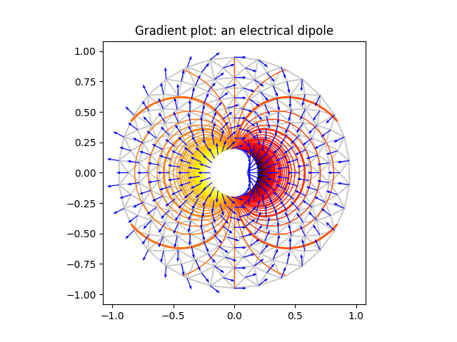
使用 matplotlib.tri.CubicTriInterpolator 演示梯度计算。
from matplotlib.tri import (Triangulation, UniformTriRefiner, CubicTriInterpolator)import matplotlib.pyplot as pltimport matplotlib.cm as cmimport numpy as np#-----------------------------------------------------------------------------# Electrical potential of a dipole#-----------------------------------------------------------------------------def dipole_potential(x, y):""" The electric dipole potential V """r_sq = x**2 + y**2theta = np.arctan2(y, x)z = np.cos(theta)/r_sqreturn (np.max(z) - z) / (np.max(z) - np.min(z))#-----------------------------------------------------------------------------# Creating a Triangulation#-----------------------------------------------------------------------------# First create the x and y coordinates of the points.n_angles = 30n_radii = 10min_radius = 0.2radii = np.linspace(min_radius, 0.95, n_radii)angles = np.linspace(0, 2 * np.pi, n_angles, endpoint=False)angles = np.repeat(angles[..., np.newaxis], n_radii, axis=1)angles[:, 1::2] += np.pi / n_anglesx = (radii*np.cos(angles)).flatten()y = (radii*np.sin(angles)).flatten()V = dipole_potential(x, y)# Create the Triangulation; no triangles specified so Delaunay triangulation# created.triang = Triangulation(x, y)# Mask off unwanted triangles.triang.set_mask(np.hypot(x[triang.triangles].mean(axis=1),y[triang.triangles].mean(axis=1))< min_radius)#-----------------------------------------------------------------------------# Refine data - interpolates the electrical potential V#-----------------------------------------------------------------------------refiner = UniformTriRefiner(triang)tri_refi, z_test_refi = refiner.refine_field(V, subdiv=3)#-----------------------------------------------------------------------------# Computes the electrical field (Ex, Ey) as gradient of electrical potential#-----------------------------------------------------------------------------tci = CubicTriInterpolator(triang, -V)# Gradient requested here at the mesh nodes but could be anywhere else:(Ex, Ey) = tci.gradient(triang.x, triang.y)E_norm = np.sqrt(Ex**2 + Ey**2)#-----------------------------------------------------------------------------# Plot the triangulation, the potential iso-contours and the vector field#-----------------------------------------------------------------------------fig, ax = plt.subplots()ax.set_aspect('equal')# Enforce the margins, and enlarge them to give room for the vectors.ax.use_sticky_edges = Falseax.margins(0.07)ax.triplot(triang, color='0.8')levels = np.arange(0., 1., 0.01)cmap = cm.get_cmap(name='hot', lut=None)ax.tricontour(tri_refi, z_test_refi, levels=levels, cmap=cmap,linewidths=[2.0, 1.0, 1.0, 1.0])# Plots direction of the electrical vector fieldax.quiver(triang.x, triang.y, Ex/E_norm, Ey/E_norm,units='xy', scale=10., zorder=3, color='blue',width=0.007, headwidth=3., headlength=4.)ax.set_title('Gradient plot: an electrical dipole')plt.show()
参考
此示例中显示了以下函数,方法,类和模块的使用:
import matplotlibmatplotlib.axes.Axes.tricontourmatplotlib.pyplot.tricontourmatplotlib.axes.Axes.triplotmatplotlib.pyplot.triplotmatplotlib.trimatplotlib.tri.Triangulationmatplotlib.tri.CubicTriInterpolatormatplotlib.tri.CubicTriInterpolator.gradientmatplotlib.tri.UniformTriRefinermatplotlib.axes.Axes.quivermatplotlib.pyplot.quiver
下载这个示例

若有收获,就点个赞吧
0 人点赞
