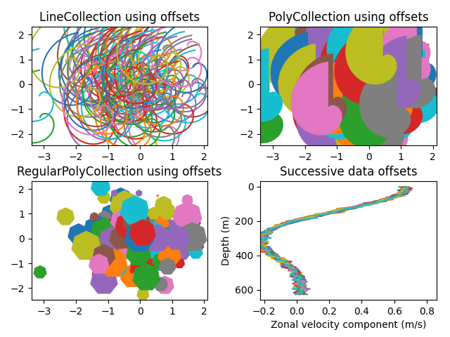
具有自动缩放功能的Line,Poly和RegularPoly Collection
对于前两个子图,我们将使用螺旋。它们的大小将以图表单位设置,而不是数据单位。它们的位置将通过使用LineCollection和PolyCollection的“偏移”和“transOffset”kwargs以数据单位设置。
第三个子图将生成正多边形,具有与前两个相同类型的缩放和定位。
最后一个子图说明了使用 “offsets =(xo,yo)”,即单个元组而不是元组列表来生成连续的偏移曲线,其中偏移量以数据单位给出。 此行为仅适用于LineCollection。
import matplotlib.pyplot as pltfrom matplotlib import collections, colors, transformsimport numpy as npnverts = 50npts = 100# Make some spiralsr = np.arange(nverts)theta = np.linspace(0, 2*np.pi, nverts)xx = r * np.sin(theta)yy = r * np.cos(theta)spiral = np.column_stack([xx, yy])# Fixing random state for reproducibilityrs = np.random.RandomState(19680801)# Make some offsetsxyo = rs.randn(npts, 2)# Make a list of colors cycling through the default series.colors = [colors.to_rgba(c)for c in plt.rcParams['axes.prop_cycle'].by_key()['color']]fig, axes = plt.subplots(2, 2)fig.subplots_adjust(top=0.92, left=0.07, right=0.97,hspace=0.3, wspace=0.3)((ax1, ax2), (ax3, ax4)) = axes # unpack the axescol = collections.LineCollection([spiral], offsets=xyo,transOffset=ax1.transData)trans = fig.dpi_scale_trans + transforms.Affine2D().scale(1.0/72.0)col.set_transform(trans) # the points to pixels transform# Note: the first argument to the collection initializer# must be a list of sequences of x,y tuples; we have only# one sequence, but we still have to put it in a list.ax1.add_collection(col, autolim=True)# autolim=True enables autoscaling. For collections with# offsets like this, it is neither efficient nor accurate,# but it is good enough to generate a plot that you can use# as a starting point. If you know beforehand the range of# x and y that you want to show, it is better to set them# explicitly, leave out the autolim kwarg (or set it to False),# and omit the 'ax1.autoscale_view()' call below.# Make a transform for the line segments such that their size is# given in points:col.set_color(colors)ax1.autoscale_view() # See comment above, after ax1.add_collection.ax1.set_title('LineCollection using offsets')# The same data as above, but fill the curves.col = collections.PolyCollection([spiral], offsets=xyo,transOffset=ax2.transData)trans = transforms.Affine2D().scale(fig.dpi/72.0)col.set_transform(trans) # the points to pixels transformax2.add_collection(col, autolim=True)col.set_color(colors)ax2.autoscale_view()ax2.set_title('PolyCollection using offsets')# 7-sided regular polygonscol = collections.RegularPolyCollection(7, sizes=np.abs(xx) * 10.0, offsets=xyo, transOffset=ax3.transData)trans = transforms.Affine2D().scale(fig.dpi / 72.0)col.set_transform(trans) # the points to pixels transformax3.add_collection(col, autolim=True)col.set_color(colors)ax3.autoscale_view()ax3.set_title('RegularPolyCollection using offsets')# Simulate a series of ocean current profiles, successively# offset by 0.1 m/s so that they form what is sometimes called# a "waterfall" plot or a "stagger" plot.nverts = 60ncurves = 20offs = (0.1, 0.0)yy = np.linspace(0, 2*np.pi, nverts)ym = np.max(yy)xx = (0.2 + (ym - yy) / ym) ** 2 * np.cos(yy - 0.4) * 0.5segs = []for i in range(ncurves):xxx = xx + 0.02*rs.randn(nverts)curve = np.column_stack([xxx, yy * 100])segs.append(curve)col = collections.LineCollection(segs, offsets=offs)ax4.add_collection(col, autolim=True)col.set_color(colors)ax4.autoscale_view()ax4.set_title('Successive data offsets')ax4.set_xlabel('Zonal velocity component (m/s)')ax4.set_ylabel('Depth (m)')# Reverse the y-axis so depth increases downwardax4.set_ylim(ax4.get_ylim()[::-1])plt.show()
参考
此示例中显示了以下函数,方法,类和模块的使用:
import matplotlibmatplotlib.figure.Figurematplotlib.collectionsmatplotlib.collections.LineCollectionmatplotlib.collections.RegularPolyCollectionmatplotlib.axes.Axes.add_collectionmatplotlib.axes.Axes.autoscale_viewmatplotlib.transforms.Affine2Dmatplotlib.transforms.Affine2D.scale
下载这个示例

若有收获,就点个赞吧
0 人点赞
