Simple linear regression is a statistical method that allows us to study relationships between two continuous variables:
- One variable, denoted
 , is regarded as the predictor, explanatory, or independent variable
 - The other variable, denoted
 , is regarded as the response, outcome, target, or dependent variable
 - The goal is to predict the value of response variable when the value of predictor variable is given
Simple linear regression gets its adjective “simple,” because it concerns the study of only one predictor variable. In contrast, multiple linear regression concerns the the general case of two or more predictor variables.多元线性回归涉及两个及两个以上的预测变量。
Linear Regression Model
Simple linear regression models the relation between predictor and response variables as follows:
where  (y-intercept)截距and
  (slope) 斜率are coefficient parameters and
  is a predicted response variable based on the predictor variable
  . If the value of coefficient parameter is positive then there is a positive relation between predictor and response variable (the value of response variable increases as the value of predictor variable increases).
The relationship between the two variables can be plotted in x-y plane as follows: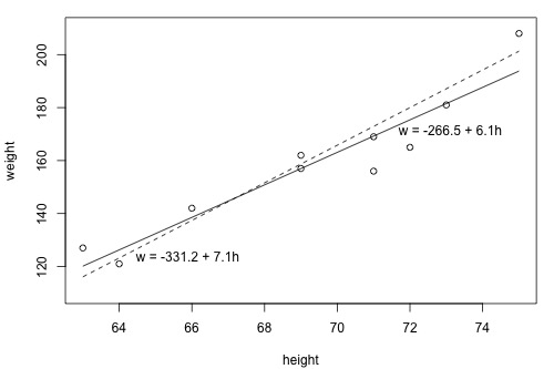
This scatter plot (dots) represent an observed pair of weight and height. Here the height is the predictor variable, and the weight is the response variable. In addition, two linear relations are suggested in this graph. You may have two natural questions from above graph:
- which line is the best line? and
- how can we find it?
What is the Best Fitting Line? 什么是最佳拟合线?
**
Let’s assume that we have a training data  which consists of n-pairs of
  and
and  .
.
The goal of parameter estimation is to estimate proper values of  and
and  . To estimate parameters, we first define the sum of square error:
 ,
,
where  is the predicted response variable. The sum of square error computes,
- the difference between the true value
 and the predicted value
  ,
, - square of the difference, and then summation of the squared difference across all training data points.
Parameter estimation finds the values for  and
and  that minimise
  and so this technique is called the least square method.
Due to the effect of squaring the differences above, linear regression is very senstitive to outliers that fall well away from the line—that is the whole fitted line will be pulled away from the non-outlying values. 由于上文方差的影响, 线性回归对outliers很敏感。
How to evaluate performance? 怎样去评估表现?
**
The parameter estimation technique suggests an evaluation technique. Accuracy does not make sense here as there are no classes; accuracy requires the independent variable value to fall either inside the class or outside the class. 不能用准确度来衡量回归,准确度只能拿来衡量分类是因为其分类依据是预测类别是否落在分类内。
The usual methods for assessing performance are
- MAE, Mean Absolute Error. It is the average of the individual errors, each one computed as the absolute value of the difference between the actual value and the predicted value. MAE of zero is a perfect fit. As there is no squared term in MAE, it does not penalise long-distance outliers as much as the regression fitting does. 计算平均绝对值误差,因为MAE中不包含平方项,因此不会过多的受噪点(long-distance outliers)影响。
- RMSE, RMSD, root mean square error. It is the square root of the average of squared errors for each value of the dependent variable, where error is the simple difference of the actual value and predicted value. It is equal to the standard deviation of the errors, and so tells you how spread out from the prediction line the actual observations are. An RMSE value of zero represents a perfect fit and there is no upper bound. 是误差的标准差,告诉你实际观测值在预测上的分布。 RMSE为零时完美拟合,没有上界。
- R-squared: the goodness of fit or coefficient of determination. It is the proportion of the dependent variable variance that is explained by a linear model. R-squared = Explained variance / Total variance. More precisely, it is 1 minus (the ratio of the sum of squared prediction error for each value of the dependent variable to the sum of squared difference from the mean for each value of the dependent variable). A value of zero says the model is only just as good as simply predicting the mean value every time, and a value of one represents a perfect fit. Minor variations include pseudo-R-squared methods and adjusted or predicted R-squared.
- Plot the predictions vs observations on a Cartesian plane and visually assess if the points appear to line up. It is a good idea to do this every time _for linear regression, in combination with quantitative measures. Are the points _close enough to the theoretical prediction = observation line? Do they fall somewhat symmetrically around that line? Are there too many points a long way off? Would a line fitted to the predictions vs observations fall close to the prediction = observation line? If it doesn’t look good, it probably isn’t.
Obviously these approaches should be applied to test data rather than training data for a proper assessment, and indeed multifold cross-validation may be applied using the quantitative performance measures above in place of accuracy.

若有收获,就点个赞吧
0 人点赞
