Accuracy, defined to be the proportion of correctly labelled tuples, is not the only measure to evaluate performance of classification. To understand the other measures, we first need to look at the confusion matrix.
Confusion Matrix (also called Error Matrix)**
A confusion matrix is a useful tool for analysing how well a classifier can recognise tuples of different classes. Given a binary classification problem, a confusion matrix is a 2 by 2 matrix where each entry indicates the number of tuples categorised by the actual class (positive or negative label in training or testing data) vs predicted class (positive or negative predicted class suggested by the classifier).
| Actual class (rows) \ Predicted class (columns) |
C1=Positive | C2=Negative |
|---|---|---|
| C1=Positive | True Positives (TP) | False Negatives (FN) |
| C2=Negative | False Positives (FP) | True Negatives (TN) |
From the confusion matrix, we can define four important measures:
- True Positive (TP): Number of positive tuples that were correctly labelled positive by the classifier
- True Negative (TN): Number of negative tuples that were correctly labelled negative by the classifier
- False Positive (FP): Number of negative tuples that were incorrectly labelled as positive by the classifier
- False negative (FN): A number of positive tuples that were incorrectly labelled as negative by the classifier
TP + TN is the number of tuples correctly labelled by the classifier (hence called True).
FP + FN is the number of tuples incorrectly labelled by the classifier (hence called False).
Note that all the FP tuples are actually N and all the FN tuples are actually P. That is, under this naming convention, the first character tells you if the classifier got it right (T) or wrong (F), and the second character tells you if the classifier predicts positive (P) or negative (N). The actual label for the tuple is not given in the name, but you can derive it.
Beware: There are several popular conventions for the layout of these matrices: sometimes postiveness is top and left as here but sometimes bottom and right; sometimes actuals are rows and predicted are columns, as here, but sometimes actuals are columns and predictions are rows. You need to pay attention to the table layout.
Example of confusion matrix (actuals are rows and predicted are columns)
- Confusion matrix for the classes buys_computer = yes and buys_computer = no
For example
- 6954: The number of positive tuples classified as positive — TP
- 412: The number of negative tuples classified as positive — FP
- 46: The number of positive tuples classified as negative — FN
- 2588: The number of negative tuples classified as negative — TN
Various evaluation measures from a confusion matrix
Let- 6954: The number of positive tuples classified as positive — TP
P = the number of tuples actually postive in the training data
- N = the number of tuples actually negative in the training data
With four primitive measures, we can define some important evaluation measures as follows: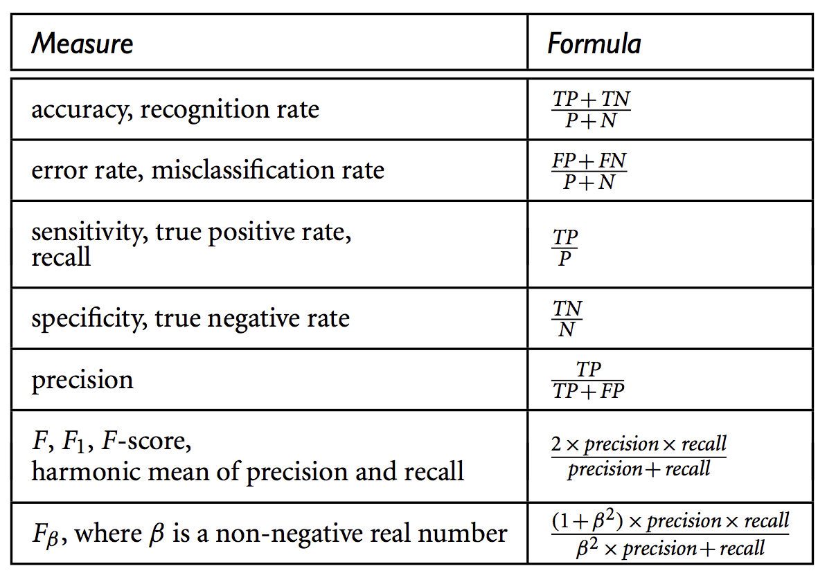
- This table shows some basic evaluation measures for classifications.
- accuracy = 1 - error rate
Class Imbalance Problem: Beware
One may wonder why we need such a range of evaluation measures. At first, the accuracy seems to be enough for a classification task, but the accuracy may not be a good way to show the performance of your classifier when the dataset is unbalanced.
An unbalanced dataset is one where the classes are not evenly distributed in the data, ie far from 50% each in the binary classification case. One class dominates the data; usually the positive class is rare.
Consider the following example that shows a confusion matrix for a cancer classification. Again, actuals are rows and predicted are columns in the table.
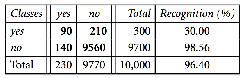
If we only care about the classifier’s accuracy, then 96.4% appears to be a good result at first glance, quite close to 100%. Wrong!
Let’s consider a classifier that we have learnt which classifies every patient as “cancer=no”. Clearly we did not need a complex data mining algorithm to learn this ridiculously simple classifier, a majority vote. In this case, we have 97.7% accuracy (9770/10000). Not bad, huh? Wrong! Our new classifier is telling us nothing, only the distribution of the classes. And note our first classifier above performed even worse than this according to accuracy, so it was unacceptably poor.
Clearly, an accuracy rate of 97% is not acceptable on this problem—a classifier with this accuracy could be correctly labelling only the noncancer tuples and misclassifying all the cancer tuples as our “cancer=no” classifier does. Instead, we need other measures, which can distinguish how well the classifier can recognise the positive tuples (cancer = yes) and how well it can recognise the negative tuples (cancer = no).
The sensitivity and specificity measures can be used, respectively, for this purpose.
For example, the sensitivity and specificity of the above example are:


Thus, we note that although the classifier has a high accuracy, it’s ability to correctly label the positive (rare) class is poor as given by its low sensitivity. It has high specificity, meaning that it can recognise negative tuples quite well. The sensitivity is much more important than specificity in this case, due to the purpose of the classification task.
But what if our classifier could deliver 100% sensitivity? Too easy: the classifier “cancer=yes” can do this. Is this a good result? No! Accuracy would be only 3%. Specificity would be 0%. Predicting all people have cancer is just as useless in practice as predicting no people have cancer.
Sensitivity and specificity are typically a tradeoff, you can maximise one by reducing the other: 100% for each is ideal (well, maybe not, due to potential overfitting discussed later), but the tradeoff between them, and whether some classifer is therefore good enough, is something for the expert to interpret with knowledge of the underlying purpose.
The precision and recall measures, originally developed for information retrieval, are also widely used in classification as alternative tradeoff quality measures:
- Precision can be thought of as a measure of exactness
- i.e., what percentage of tuples classified as positive are actually such
- Recall (equivalent to sensitivity, above) is a measure of completeness
- i.e., what percentage of positive tuples are classified as such
Often precision and recall are combined into an F1-score, which is the harmonic mean of the precision and recall. It might also be called simply f-score, or f-measure. See the table above for its formulation. Maximising f-score is useful because it provides a single measure, and takes account of potentially unbalanced data by focusing on the postive class, but it emphasises a particular relationship between right and wrong predictions. Is this the right quality measure for your classification task? Or not?
ACTION: Calculate precision, recall and f-measure for the cancer classification confusion matrix above as well as for the classifiers “cancer=yes” (which classifies every tuple as positive) and “cancer=no” (which classifies every tuple as negative). Comment on the interpretation of f-measure for this problem. A worked solution is here: Solution to Exercise: Evaluation measures
Key message: Always consider whether your measure of performance is appropriate for your problem. Choose an appropriate measure which might be influenced by the practice in the domain of application. Always consider how your performance compares to a dumb classifier which might be 50% accuracy for a balanced dataset but something else for unbalanced data.

若有收获,就点个赞吧
0 人点赞
