Zero-probability problem
Naïve Bayesian prediction requires each class conditional probability to be non-zero, as otherwise the predicted probability will be zero.
Example
Let’s assume that we extract following two tables for _student _and _credit _attributes from a customer history, where each entry represents a number of customers:
| Buy computer \ Student | Yes | No |
|---|---|---|
| Yes | 0 | 5 |
| No | 3 | 7 |
| Buy computer \ credit | Fair | Excellent |
|---|---|---|
| Yes | 4 | 1 |
| No | 6 | 4 |
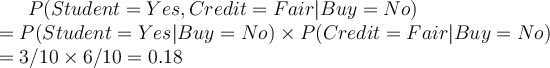
Using naive Bayes, let’s classify the probability of a student with fair credit buying a computer. First, we need to compute the likelihood: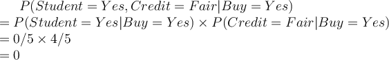
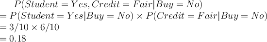
Therefore, the classifier will classify that the student will not buy a computer irrespective of the prior. This is because no student has bought a computer ever before. In other words, the likelihood of student buying a computer:  , indicates irrespective of the other attributes, the classifier will always classify a student tuple as not buy a computer. During the classification of an unlabelled tuple, all the other attributes have no effect if the student _attribute is _Yes. This is not wrong, but inconvenient, as in some cases, the other attributes may have a different opinion to contribute to the classification of the tuple.
Laplace correction
To avoid the zero probability in the likelihood, we can simply add a small constant to the summary table as follows:
| Buy computer \ Student | Yes | No |
|---|---|---|
| Yes | 0+ |
5+ |
| No | 3 | 7 |
If we let  , which is the usual value, then the likelihoods of naive Bayes are:
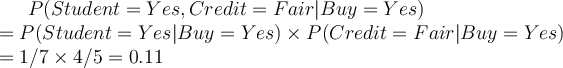
Using the Laplacian correction with  of 1, we pretend that we have 1 more tuple for each possible value for Student (i.e., Yes and No, here) but we only pretend this while computing the likelihood factors for the attribute and class combination which has a zero count in the data for at least one of its values.
Likelihood for alternative(non-zero count) values of the affected attribute are also affected, but this will come into play when we are predicting a _different _customer at a different time: e.g.
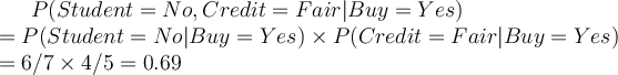
The likelihood for the other class (for the same student with fair credit) is unchanged as before:
The “corrected” probability estimates are close to their “uncorrected” counterparts, yet the zero probability value is avoided.

若有收获,就点个赞吧
0 人点赞
