Author:Sijie Yan, Yuanjun Xiong and Dahua Lin 论文原文:Spatial Temporal Graph Convolutional Networks for Skeleton-Based Action Recognition 博客参考:St-gcn 动作识别 理论+源码分析(Pytorch) 代码实现:https://github.com/yongqyu/st-gcn-pytorch
Introduction
In this work, we propose a novel model of dynamic skeletons called Spatial Temporal Graph Convolutional Networks (ST-GCN), which moves beyond the limitations of previous methods by automatically learning both the spatial and temporal patterns from data. On two large datasets, Kinetics and NTU-RGBD, it achieves substantial improvements over mainstream methods.
那么什么是 dynamic skeletons 呢?那么如何体现 automatically 以及 spatial and temporal 的呢?(并且其他方法为何不 automatical?) mainstream: 肯定是后面进行对比的方法咯,在对比中体现巨大的性能提升。
Multiple modalities of human action
Human action recognition has become an active research area in recent years, as it plays a significant role in video understanding. In general, human action can be recognized from multiple modalities(Simonyan and Zisserman 2014; Tran et al. 2015; Wang, Qiao, and Tang 2015; Wang et al. 2016; Zhao et al. 2017), such as appearance, depth, optical flows, and body skeletons (Du, Wang, and Wang 2015; Liu et al. 2016).
modalities: 模式 对于单张图片的算法,最高境界就是图像的理解和推理;视频算法,当然也是希望最终实现视频的理解。 视频的建模可以粗分为三类:基于二维图像,基于深度图像,基于光流,基于人体骨架。
The weakless of previous methods
The dynamic skeleton modality can be naturally represented by a time series of human joint locations, in the form of 2D or 3D coordinates. Human actions can then be recognized by analyzing the motion patterns thereof. Earlier methods of using skeletons for action recognition simply employ the joint coordinates at individual time steps to form feature vectors, and apply temporal analysis thereon (Wang et al. 2012; Fernando et al. 2015). The capability of these methods is limited as they do not explicitly exploit the spatial relationships among the joints, which are crucial for understanding human actions.
之前的方法,只是将不同帧的关节点组成向量,然后在时间域进行组合学习。这种方法并没有考虑到人体关节点本身的连接关系等 => 由此可知,后面将会介绍如何引入关节点的空间域关系建模。
Recently, new methods that attempt to leverage the natural connections between joints have been developed (Shahroudy et al. 2016; Du, Wang, and Wang 2015). These methods show encouraging improvement, which suggests the significance of the connectivity. Yet, most existing methods rely on hand-crafted parts or rules to analyze the spatial patterns. As a result, the models devised for a specific application are difficult to be generalized to others.
考虑了人体本身关节点的连接关系,能够提高网络性能;但是不利于移植到其它应用上。???
To move beyond such limitations, we need a new method that can automatically capture the patterns embedded in the spatial configuration of the joints as well as their temporal dynamics. This is the strength of deep neural networks. However, as mentioned, the skeletons are in the form of graphs instead of a 2D or 3D grids, which makes it difficult to use proven models like convolutional networks.
前面对图卷积的研究,产生了一系列的应用:such as image classification (Bruna et al. 2014), document classification (Defferrard, Bresson, and Vandergheynst 2016), and semi-supervised learning (Kipf and Welling 2017). 但是都是以固定图作为输入。
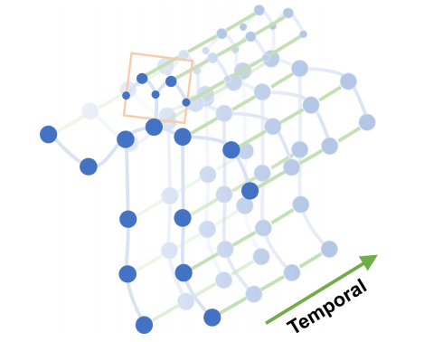
Fig (1) : The spatial temporal graph of a skeleton sequence
used in this work where the proposed ST-GCN operate on
This work’s advantages
There are two types of edges, namely the spatial edges that conform to the natural connectivity of joints and the temporal edges that connect the same joints across consecutive time steps. Multiple layers of spatial temporal graph convolution are constructed thereon, which allow information to be integrated along both the spatial and the temporal dimension.
The hierarchical nature of ST-GCN eliminates the need of hand-crafted part assignment or traversal rules.
如何理解 hierarchical nature?(层次化本质)也即是说 hierarchical nature 实现了 automatically learning. 从另一方面,这句话表示其他方法需要进行 hand-crafted part assignment or traversal rules。
This (hierarchical nature…) not only leads to greater expressive power and thus higher performance (as shown in our experiments), but also makes it easy to generalize to different contexts. Upon the generic GCN formulation, we also study new strategies to design graph convolution kernels, with inspirations from image models.
可以看到此处的 gcn 与之前阅读的几篇 gcn 文章的核设计将会有所差异。
The major contributions of this work lie in three aspects: 1) We propose ST-GCN, a generic graph-based formulation for modeling dynamic skeletons, which is the first that applies graph-based neural networks for this task. 2) We propose several principles in designing convolution kernels in ST-GCN to meet the specific demands in skeleton modeling. 3) On two large scale datasets for skeleton-based action recognition, the proposed model achieves superior performance as compared to previous methods using hand-crafted parts or traversal rules, with considerably less effort in manual design. The code and models of ST-GCN are made publicly available.
Related work
Introduction 里面比较宽泛地介绍了 human action recognition 任务,在 Related work 里面将进行细化,将焦点集中于 Skeleton Based. 两者都是综述性质的?
Neural Networks on Graphs
Generalizing neural networks to data with graph structures is an emerging topic in deep learning research.
The discussed neural network architectures include both recurrent neural networks (Tai, Socher, and Manning 2015; Van Oord, Kalchbrenner, and Kavukcuoglu 2016) and convolutional neural networks (CNNs) (Bruna et al. 2014; Henaff, Bruna, and LeCun 2015; Duvenaud et al. 2015; Li et al. 2016; Defferrard, Bresson, and Vandergheynst 2016). This work is more related to the generalization of CNNs, or graph convolutional networks (GCNs). 神经网络有很多类型,之前有一个误解:所有的这些目前主流的神经网络都是 CNN. 其实并且如何,它们的差异还是很大的。机器学习
深度学习
神经网络
CNNs,每一个概念都是一个包含的关系。
The principle of constructing GCNs on graph generally follows two streams: 1) the spectral perspective, where the locality of the graph convolution is considered in the form of spectral analysis (Henaff, Bruna, and LeCun 2015; Duvenaud et al. 2015; Li et al. 2016; Kipf and Welling 2017); 2) the spatial perspective, where the convolution filters are applied directly on the graph nodes and their neighbors (Bruna et al. 2014; Niepert, Ahmed, and Kutzkov 2016). This work follows the spirit of the second stream. We construct the CNN filters on the spatial domain, by limiting the application of each filter to the 1-neighbor of each node.
对于 Graph convolution 的构建可以从谱分析和空间的角度进行展开。之前貌似在哪里看到过图卷积利用拉普拉斯矩阵进行谱分析啥的(其也是研究图的)。 本文采用的是直接从空间域的方式来构建卷积。
Skeleton Based Action Recognition
Skeleton and joint trajectories(轨迹) of human bodies are robust to illumination(光照) change and scene variation, and they are easy to obtain owing to the highly accurate depth sensors or pose estimation algorithms (Shotton et al. 2011; Cao et al. 2017a). There is thus a broad array of skeleton based action recognition approaches.
The approaches can be categorized into handcrafted feature based methods and deep learning methods. The first type of approaches design several handcrafted features to capture the dynamics of joint motion. These could be covariance matrices of joint trajectories (Hussein et al. 2013), relative positions of joints (Wang et al. 2012), or rotations and translations between body parts (Vemulapalli, Arrate, and Chellappa 2014).
传统的方法,没有了解过。(顺便把它当成一片综述进行阅读罗~)
The recent success of deep learning has lead to the surge of deep learning based skeleton modeling methods. These works have been using recurrent neural networks (Shahroudy et al. 2016; Zhu et al. 2016; Liu et al. 2016; Zhang, Liu, and Xiao 2017) and temporal CNNs (Li et al. 2017; Ke et al. 2017; Kim and Reiter 2017) to learn action recognition models in an end-to-end manner. Among these approaches, many have emphasized the importance of modeling the joints within parts of human bodies. But these parts are usually explicitly assigned using domain knowledge.
深度学习的方法,采用 RNN(采用LSTM测试效果较差,不知是否有注意的地方?),temporal CNNs(之前毕设采用过,效果还可以,其思想就是将关键点序列组合成为图像的形式) 本段最后一句:Among these approaches…所谓何意?1、对人体关节点空间建模是重要的;2、先前的方法通过领域知识显式分配(?)
Our ST-GCN is the first to apply graph CNNs to the task of skeleton based action recognition. It differentiates from previous approaches in that it can learn the part information implicitly by harnessing locality of graph convolution together with the temporal dynamics. By eliminating the need for manual part assignment, the model is easier to design and potent to learn better action representations.
给我的感觉,貌似是,对于人体的关键点空间连接无需进行显式分配?比如说不需要关键点的邻接矩阵啥的?
Spatial Temporal Graph ConvNet
When performing activities, human joints move in small local groups, known as “body parts”. Existing approaches for skeleton based action recognition have verified the effectiveness of introducing body parts in the modeling(Shahroudy et al. 2016; Liu et al. 2016; Zhang, Liu, and Xiao 2017).
“body parts”:层次显然高于关键点。在前面并不明白“body parts”是什么从而将关键点与之等同,所以产生了一些疑惑。(网络结构设计很重要,但是值得一提的是很多时候将会产生冗余设计)
We argue that the improvement is largely due to that parts restrict the modeling of joints trajectories within “local regions” compared with the whole skeleton, thus forming a hierarchical representation of the skeleton sequences.
我们认为,改进的主要原因是部分限制了建模的关节轨迹在“局部区域”,而不是整个骨架,从而形成了骨骼序列的层次表示。
In tasks such as image object recognition, the hierarchical representation and lo__cality are usually achieved by the intrinsic(固有的) properties of convolutional neural networks (Krizhevsky, Sutskever, and Hinton 2012), rather than manually assigning object parts. It motivates us to introduce the appealing property of CNNs to skeleton based action recognition. The result of this attempt is the ST-GCN model.
这里提到了 CNNs 的层次化表征以及局部性。
Skeleton based data can be obtained from motion-capture devices or pose estimation algorithms from videos. Usually the data is a sequence of frames, each frame will have a set of joint coordinates. Given the sequences of body joints in the form of 2D or 3D coordinates, we construct a spatial temporal graph with the joints as graph nodes and natural connectivities in both human body structures and time as graph edges. The input to the ST-GCN is therefore the joint coordinate vectors on the graph nodes. This can be considered as an analog(类似物) to image based CNNs where the input is formed by pixel intensity(强度) vectors residing on the 2D image grid. Multiple layers of spatial-temporal graph convolution operations will be applied on the input data and generating higher-level feature maps on the graph. It will then be classified by the standard SoftMax classifier to the corresponding action category. The whole model is trained in an end-to-end manner with backpropagation. We will now go over the components in the ST-GCN model.
类比于 CNNs 进行阐述。
Skeleton Graph Construction
A skeleton sequence is usually represented by 2D or 3D coordinates of each human joint in each frame. Previous work using convolution for skeleton action recognition (Kim and Reiter 2017) concatenates coordinate vectors of all joints to form a single feature vector per frame. In our work, we utilize the spatial temporal graph to form hierarchical representation of the skeleton sequences.
Particularly, we construct an undirected spatial temporal graph G = (V, E) on a skeleton sequence with N joints and T frames featuring both intra-body and inter-frame connection. In this graph, the node set  includes the all the joints in a skeleton sequence. As ST-GCN’s input, the feature vector on a node
  consists of coordinate vectors, as well as estimation confidence, of the
  joint on frame t. We construct the spatial temporal graph on the skeleton sequences in two steps. First, the joints within one frame are connected with edges according to the connectivity of human body structure, which is illustrated in Fig. 1. Then each joint will be connected to the same joint in the consecutive frame. The connections in this setup are thus naturally defined without the manual part assignment.
First 和 then 就是所说的两步吧。“in this setup”是包括两步,还是只包括后面的一步?从后面看是两步都是(但是代码貌似看起来只包括了第二步)?
This also enables the network architecture to work on datasets with different number of joints or joint connectivities. For example, on the Kinetics dataset, we use the 2D pose estimation results from the OpenPose (Cao et al. 2017b) toolbox which outputs 18 joints, while on the NTURGB+D dataset (Shahroudy et al. 2016) we use 3D joint tracking results as input, which produces 25 joints. The STGCN can operate in both situations and provide consistent superior performance. An example of the constructed spatial temporal graph is illustrated in Fig. 1.
Formally, the edge set E is composed of two subsets, the first subset depicts the intra-skeleton connection at each frame, denoted as  , where H is the set of naturally connected human body joints. The second subset contains the inter-frame edges, which connect the same joints in consecutive frames as
  . Therefore all edges in
  for one particular joint
  will represent its trajectory over time.
非常简单的表征公式。
Spatial Graph Convolutional Neural Network
这才是本文的重点所在,即作者是如何设计得 ST-GCN?
Before we dive into the full-fledged ST-GCN, we first look at the graph CNN model within one single frame. In this case, on a single frame at time τ , there will be N joint nodes  , along with the skeleton edges
  .
.
图的表征,后面推导会用。
Recall the definition of convolution operation on the 2D natural images or feature maps, which can be both treated as 2D grids. The output feature map of a convolution operation is again a 2D grid. With stride 1 and appropriate padding, the output feature maps can have the same size as the input feature maps. We will assume this condition in the following discussion. Given a convolution operator with the kernel size of  , and an input feature map
  with the number of channels c. The output value for a single channel at the spatial location x can be written as
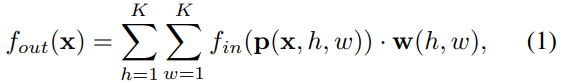
p is sampling function, w is weight function.(Dai et al. 2017).
卷积操作介绍就算了…但是可以从卷积操作中抽像出更为本质的东西,从而使其能够进行一个推广。 这个公式表示的是什么呢?它想表达的是:在只考虑输出单channel 的条件下,输入一个 feature map 以及一个指定的坐标,那么以该坐标为中心的邻域(包括 channel 维度的数据)与卷积核进行一次运算产生一个输出。
The convolution operation on graphs is then defined by extending the formulation above to the cases where the input features map resides on a spatial graph  . That is, the feature map
  has a vector on each node of the graph. The next step of the extension is to redefine the sampling function p and the weight function w.
Sampling function
On images, the sampling function  is defined on the neighboring pixels with respect to the center location x. On graphs, we can similarly define the sampling function on the neighbor set
  of a node
  . Here
  denotes the minimum length of any path from
  to
to  . Thus the sampling function
  can be written as
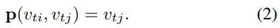
In this work we use D = 1 for all cases, that is, the 1- neighbor set of joint nodes. The higher number of D is left for future works.
还留一手? 采样之后还包括 root node 吗?看公式貌似是没有包括的。但是从后面类比于 2D Grid 看出,是包括 root node 的。
Weight function
Compared with the sampling function, the weight function is trickier to define. In 2D convolution, a rigid grid naturally exists around the center location. So pixels within the neighbor can have a fixed spatial order. The weight function can then be implemented by indexing a tensor of (c, K, K) dimensions according to the spatial order. For general graphs like the one we just constructed, there is no such implicit arrangement. The solution to this problem is first investigated in (Niepert, Ahmed, and Kutzkov 2016), where the order is defined by a graph labeling process in the neighbor graph around the root node. We follow this idea to construct our weight function.
该论文需要仔细阅读一下。 然后,可以看到,论文认为要实现图卷积主要问题还是如何实现节点类似图像 2D Grids 的组织。
Instead of giving every neighbor node a unique labeling, we simplify the process by partitioning the neighbor set  of a joint node
  into a fixed number of K subsets, where each subset has a numeric label. Thus we can have a mapping
  which maps a node in the neighborhood to its subset label. The weight function
  can be implemented by indexing a tensor of (c, K) dimension or
We will discuss several partitioning strategies after.
为何要固定 K 呢?那么如何处理一些邻节点数不等于 K 的节点呢?
Spatial Graph Convolution
With the refined sampling function and weight function, we now rewrite Eq. 1 in terms of graph convolution as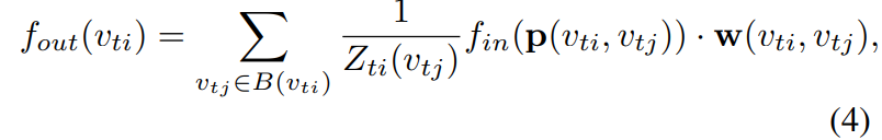
where the normalizing term  equals the cardinality(基数) of the corresponding subset. This term is added to balance the contributions of different subsets to the output. Substituting Eq. 2 and Eq. 3 into Eq. 4, we arrive at
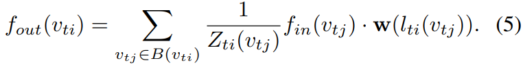
It is worth noting this formulation can resemble the standard 2D convolution if we treat a image as a regular 2D grid. For example, to resemble a 3×3 convolution operation, we have a neighbor of 9 pixels in the 3 × 3 grid centered on a pixel. The neighbor set should then be partitioned into 9 subsets, each having one pixel.
It is worth noting: 值得注意的是
表达的意思是集合的大小,即其所说的基数(集合里面的概念)
Spatial Temporal Modeling
Having formulated spatial graph CNN, we now advance to the task of modeling the spatial temporal dynamics within skeleton sequence. Recall that in the construction of the graph, the temporal aspect of the graph is constructed by connecting the same joints across consecutive frames. This enable us to define a very simple strategy to extend the spatial graph CNN to the spatial temporal domain. That is, we extend the concept of neighborhood to also include temporally connected joints as
开始以为公式有点小错误(后面的是
),但是后面才发现这个公式没有问题,计算关键点距离,不考虑时域上的变换,只考虑空间关系。
The parameter  controls the temporal range to be included in the neighbor graph and can thus be called the temporal kernel size. To complete the convolution operation on the spatial temporal graph, we also need the sampling function, which is the same as the spatial only case, and the weight function, or in particular, the labeling map
  . Because the temporal axis is well-ordered, we directly modify the label map
  for a spatial temporal neighborhood rooted at
  to be
to be
where  is the label map for the single frame case at
  . In this way, we have a well-defined convolution operation on the constructed spatial temporal graphs.
看看看,主要就是要实现 label 的分配。对于不同时间上的,通过公式的后半部分进行区分。这样就将原来的
,变为
. 也就是说上面的公式是在原来
基础上进行修改之后的,将首帧赋值
,后面每增加一帧,则对应在上一帧基础上进行平移
. 值得一提的是,目前为止,在计算过程中,并不会使得图变小,无论经过多少次卷积,图还是原来一样大。(当然,节点的 feature 被当作 channel 进行处理。(但是可以实现 channel 的改变)
Partition Strategies
Given the high-level formulation of spatial temporal graph convolution, it is important to design a partitioning strategy to implement the label map  . In this work we explore several partition strategies. For simplicity, we only discuss the cases in a single frame because they can be naturally extended to the spatial-temporal domain using Eq. 7.
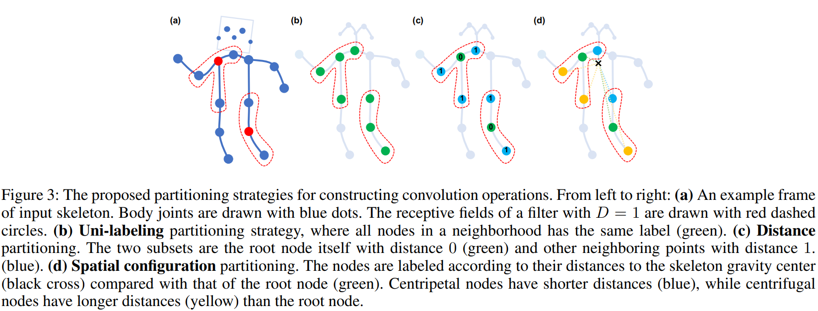
Uni-labeling
The simplest and most straight forward partition strategy is to have subset, which is the whole neighbor set itself. In this strategy, feature vectors on every neighboring node will have a inner product with the same weight vector. Actually, this strategy resembles the propagation rule introduced in (Kipf and Welling 2017). It has an obvious drawback that in the single frame case, using this strategy is equivalent to computing the inner product between the weight vector and the average feature vector of all neighboring nodes. This is suboptimal for skeleton sequence classification as the local differential properties could be lost in this operation. Formally, we have K = 1 and  .
.
Distance partitioning
Another natural partitioning strategy is to partition the neighbor set according to the nodes’ distance  to the root node
  . In this work, because we set D = 1, the neighbor set will then be separated into two subsets, where d = 0 refers to the root node itself and remaining neighbor nodes are in the d = 1 subset. Thus we will have two different weight vectors and they are capable of modeling local differential properties such as the relative translation between joints. Formally, we have K = 2 and
  .
.
Spatial configuration partitioning
Since the body skeleton is spatially localized, we can still utilize this specific spatial configuration in the partitioning process. We design a strategy to divide the neighbor set into three subsets: 1) the root node itself; 2)centripetal(向心) group: the neighboring nodes that are closer to the gravity center of the skeleton than the root node; 3) otherwise the centrifugal(离心) group. Here the average coordinate of all joints in the skeleton at a frame is treated as its gravity center. This strategy is inspired by the fact that motions of body parts can be broadly categorized as concentric and eccentric motions. Formally, we have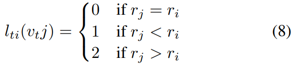
这里考虑向心和离心只需要考虑当前帧,前后帧的即使可能出现了向心和离心的变换也仍旧按照当前帧的分类进行处理。(见公式(7))
where  is the average distance from gravity center to joint i over all frames in the training set. Visualization of the three partitioning strategies is shown in Fig. 3. We will empirically examine the proposed partioning strategies on skeleton based action recognition experiments. It is expected that a more advanced partitioning strategy will lead to better modeling capacity and recognition performance.
这种方式中心和关键点的平均距离不好计算…根据前面的描述,关键点的分组貌似是动态的,但是根据此处的描述关键点分组又是静态的。
Learnable edge importance weighting
Although joints move in groups when people are performing actions, one joint could appear in multiple body parts. These appearances, however, should have different importance in modeling the dynamics of these parts. In this sense, we add a learnable mask M on every layer of spatial temporal graph convolution. The mask will scale the contribution of a node’s feature to its neighboring nodes based on the learned importance weight of each spatial graph edge in  . Empirically we find adding this mask can further improve the recognition performance of ST-GCN. It is also possible to have a data dependent attention map for this sake. We leave this to future works.
此处就是讲述注意力机制了。(通过加权实现啊)
Implementing ST-GCN
The implementation of graph-based convolution is not as straightforward as 2D or 3D convolution. Here we provide details on implementing ST-GCN for skeleton based action recognition.
We adopt a similar implementation of graph convolution as in (Kipf and Welling 2017). The intra-body connections of joints within a single frame are represented by an adjacency matrix A and an identity matrix I representing self-connections. In the single frame case, ST-GCN with the first partitioning strategy can be implemented with the following formula (Kipf and Welling 2017)
前面有讲过原理分析。将所谓的卷积转为了矩阵乘法。那感觉和之前的GCN有啥区别呢?基本上还是和之前的一样啊?(卷积的实现有些也是转为矩阵乘法啊。)从这里来看的话,前面的公式就是从更抽象的角度来描述了解决方式
where  Here the weight vectors of multiple output channels are stacked to form the weight matrix W. In practice, under the spatial temporal cases, we can represent the input feature map as a tensor of (C, V, T) dimensions. The graph convolution is implemented by performing a 1 × Γ standard 2D convolution and multiplies the resulting tensor with the normalized adjacency matrix
  on the second dimension.
节点的特征在这里都体现在 channel 里面,即:它的特征由一个向量组成。
For partitioning strategies with multiple subsets, i.e., distance partitioning and spatial configuration partitioning, we again utilize this implementation. But note now the adjacency matrix is dismantled into several matrixes  where
where  . For example in the distance partitioning strategy,
  and
and  . The Eq. 9 is transformed into
这种形式是如何实现的呢?这需要考虑到前面的

where similarly  . Here we set α = 0.001 to avoid empty rows in
  .
.
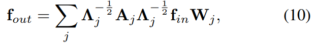
It is straightforward to implement the learnable edge importance weighting. For each adjacency matrix, we accompany it with a learnable weight matrix M. And we substitute the matrix A + I in Eq. 9 and  in
in  in Eq. 10 with
  and
and  , respectively. Here
  denotes element-wise product between two matrixes. The mask M is initialized as an all-one matrix.
Network architecture and training
Since the ST-GCN share weights on different nodes, it is important to keep the scale of input data consistent on different joints. In our experiments, we first feed input skeletons to a batch normalization layer to normalize data. The ST-GCN model is composed of 9 layers of spatial temporal graph convolution operators (ST-GCN units). The first three layers have 64 channels for output. The follow three layers have 128 channels for output. And the last three layers have 256 channels for output. These layers have 9 temporal kernel size. The Resnet mechanism is applied on each ST-GCN unit. And we randomly dropout the features at 0.5 probability after each STGCN unit to avoid overfitting. The strides of the 4-th and the 7-th temporal convolution layers are set to 2 as pooling layer. After that, a global pooling was performed on the resulting tensor to get a 256 dimension feature vector for each sequence. Finally, we feed them to a SoftMax classifier. Tdecay the lehe models are learned using stochastic gradient descent with a learning rate of 0.01. We arning rate by 0.1 after every 10 epochs. To avoid overfitting, we perform two kinds of augmentation to replace dropout layers when training on the Kinetics dataset (Kay et al. 2017). First, to simulate the camera movement, we perform random affine transformations on the skeleton sequences of all frames. Particularly, from the first frame to the last frame, we select a few fixed angle, translation and scaling factors as candidates and then randomly sampled two combinations of three factors to generate an affine transformation. This transformation is interpolated for intermediate frames to generate a effect as if we smoothly move the view point during playback. We name this augmentation as random moving. Second, we randomly sample fragments from the original skeleton sequences in training and use all frames in the test. Global pooling at the top of the network enables the network to handle the input sequences with indefinite length.
Experiments
This Kinetics dataset provides only raw video clips without skeleton data. In this work we are focusing on skeleton based action recognition, so we use the estimated joint locations in the pixel coordinate system as our input and discard the raw RGB frames. To obtain the joint locations, we first resize all videos to the resolution of 340 × 256 and convert the frame rate to 30 FPS. Then we use the public available OpenPose (Cao et al. 2017b) toolbox to estimate the location of 18 joints on every frame of the clips. The toolbox gives 2D coordinates (X, Y ) in the pixel coordinate system and confidence scores C for the 18 human joints. We thus represent each joint with a tuple of (X, Y, C__) and a skeleton frame is recorded as an array of 18 tuples. For the multi-person cases, we select 2 people with the highest average joint confidence in each clip. In this way, one clip with T frames is transformed into a skeleton sequence of these tuples. In practice, we represent the clips with tensors of (3, T, 18, 2) dimensions. For simplicity, we pad every clip by replaying the sequence from the start to have T = 300. We will release the estimated joint locations on Kinetics for reproducing the results.
Ablation Study
Spatial temporal graph convolution. First, we evaluate the necessity of using spatial temporal graph convolution operation. We use a baseline network architecture (Kim and Reiter 2017) where all spatial temporal convolutions are replaced by only temporal convolution. That is, we concatenate all input joint locations to form the input features at each frame t. The temporal convolution will then operate on this input and convolves over time. We call this model “baseline TCN”. This kind of recognition models is known to work well on constraint dataset such as NTU-RGB+D (Kim and Reiter 2017). Seen from Table 1, models with spatial temporal graph convolution, with reasonable partitioning strategies, consistently outperform the baseline model on Kinetics. Actually, this temporal convolution is equivalent to spatial temporal graph convolution with unshared weights on a fully connected joint graph. So the major difference between the baseline model and ST-GCN models are the sparse natural connections and shared weights in convolution operation. Additionally, we evaluate an intermediate model between the baseline model and ST-GCN, referred as “local convolution”. In this model we use the sparse joint graph as ST-GCN, but use convolution filters with unshared weights. We believe the better performance of ST-GCN based models could justify the power of the spatial temporal graph convolution in skeleton based action recognition.
Partition strategies. In this work we present three partitioning strategies: 1) uni-labeling; 2) distance partitioning; and 3) spatial configuration partitioning. We evaluate the performance of ST-GCN with these partitioning strategies. The results are summarized in Table 1. We observe that partitioning with multiple subsets is generally much better than uni-labeling. This is in accordance with the obvious problem of uni-labeling that it is equivalent to simply averaging features before the convolution operation. Given this observation, we experiment with an intermediate between the distance partitioning and uni-labeling, referred to as “distance partitioning”. In this setting we bind the weights of the two subsets in distance partitioning to be different only by a scaling factor −1, or  . This setting still achieves better performance than uni-labeling, which again demonstrate the importance of the partitioning with multiple subsets. Among multi-subset partitioning strategies, the spatial configuration partitioning achieves better performance. This corroborates our motivation in designing this strategy, which takes into consideration the concentric and eccentric motion patterns. Based on these observations, we use the spatial configuration partitioning strategy in the following experiments.
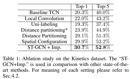
Learnable edge importance weighting. Another component in ST-GCN is the learnable edge importance weighting. We experiment with adding this component on the ST-GCN model with spatial configuration partitioning. This is referred to as “ST-GCN+Imp.” in Table 1. Given the high performing vanilla ST-GCN, this component is still able to raise the recognition performance by more than 1 percent. *Recall that this component is inspired by the fact that joints in different parts have different importances. It is verified that the ST-GCN model can now learn to express the joint importance and improve the recognition performance. Based on this observation, we always use this component with STGCN in comparison with other state-of-the-art models.
Comparison with State of the Arts
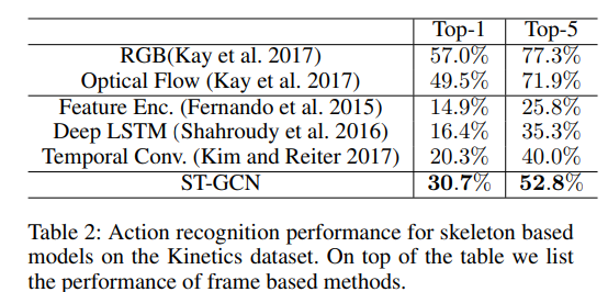
Kinetics. On Kinetics, we compare with three characteristic approaches for skeleton based action recognition. The first is the feature encoding approach on hand-crafted features (Fernando et al. 2015), referred to as “Feature Encoding” in Table 2. We also implemented two deep learning based approaches on Kinetics, i.e. Deep LSTM (Shahroudy et al. 2016) and Temporal ConvNet (Kim and Reiter 2017). We compare the approaches’ recognition performance in terms of top-1 and top-5 accuracies. In Table 2, ST-GCN is able to outperform previous representative approaches. For references, we list the performance of using RGB frames and optical flow for recognition as reported in (Kay et al. 2017).
相对于最好的使用 RGB 和光流的方法还是有差距的。
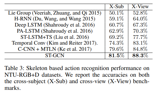
NTU-RGB+D. The NTU-RGB+D dataset is captured in a constraint environment, which allows for methods that require well stabilized skeleton sequences to work well. We also compare our ST-GCN model with the previous state-ofthe-art methods on this dataset. Due to the constraint nature of this dataset, we do not use any data augmentation when training ST-GCN models. We follow the standard practice in literature to report cross-subject (X-Sub) and crossview (X-View) recognition performance in terms of top1 classification accuracies. The compared methods include Lie Group (Veeriah, Zhuang, and Qi 2015), Hierarchical RNN (Du, Wang, and Wang 2015), Deep LSTM (Shahroudy et al. 2016), Part-Aware LSTM (PA-LSTM) (Shahroudy et al. 2016), Spatial Temporal LSTM with Trust Gates (STLSTM+TS) (Liu et al. 2016), Temporal Convolutional Neural Networks (Temporal Conv.) (Kim and Reiter 2017), and Clips CNN + Multi-task learning (C-CNN+MTLN) (Ke et al. 2017). Our ST-GCN model, with rather simple architecture and no data augmentation as used in (Kim and Reiter 2017; Ke et al. 2017), is able to outperform previous stateof-the-art approaches on this dataset.
总结
本文就是在之前图卷积的基础上,进一步进行改进。本文主要特点是:1、定义了时间域上的邻接点(见公式6),从而引出ST-GCN;2、加入可学习参数,使得不同节点权重不同(类似注意力机制);3、尝试了不同邻接点策略;4、取得了不错的分类成绩;
代码分析
由 ConvTemporalGraphical 以及 tcn 组成 st-gcn
ConvTemporalGraphical
The based unit of graph convolutional networks.
class ConvTemporalGraphical(nn.Module):def __init__(self,in_channels,out_channels,kernel_size,t_kernel_size=1,t_stride=1,t_padding=0,t_dilation=1,bias=True):super().__init__()self.kernel_size = kernel_sizeself.conv = nn.Conv2d(in_channels,out_channels * kernel_size,kernel_size=(t_kernel_size, 1),padding=(t_padding, 0),stride=(t_stride, 1),dilation=(t_dilation, 1),bias=bias)def forward(self, x, A):assert A.size(0) == self.kernel_sizex = self.conv(x)n, kc, t, v = x.size()x = x.view(n, self.kernel_size, kc//self.kernel_size, t, v)# Einstein index summationx = torch.einsum('nkctv,kvw->nctw', (x, A))return x.contiguous(), A
这里采用了爱因斯坦指标求和,借助它可以实现很复杂的操作
- 首先爱因斯坦指标求和进行计算的时候,不用考虑矩阵的位置。然后就是对角矩阵在做乘法操作的时候可以与其他矩阵交换顺序。
- 根据公式(10)来理解为何要写成这种形式。事实上对公式10的矩阵乘法可以进一步展开,在展开之前记性如下化简:记
,
,则(10)简化为
如果再考虑 batch size 和 channel,那么就可以写作:
(下标可能并没有和上面的对应)
- 这里貌似当 **t_kernel_size = 1 时,并没有将 temporal 节点考虑进来**。
我们要完成的任务:
- 由于节点被分类了,所以对于
以及
也要进行拆分,其中
可以直接从
产生,所以只需要考虑
的组织即可。
- 然后
可以被当成一个整体进行处理(这正是代码中所采用的方法,在获取 A 的同时对其进行归一化)。(参考后面的函数)
这里有两个要点:1、拆分是如何表示的?2、如何引入参数 W ?
- 对于1:在构造邻接矩阵的时候,作者生成多个矩阵来表示拆分关系,比如在 Distance partitioning 中,作者将距离为 0 和距离为 1 的节点分别生成两个矩阵产生 A.shape = (2,18,18)( 对于第三种策略中合并了a_root + a_close倒是没有看懂是想干嘛?)
- 对于2:作者采用了
卷积整合了 channel 信息,并将产生输出 channel 与 A.shape[0] 对应,从而使得后面可以对该维度进行爱因斯坦指标求和。(由于是
也就是多个
,所以通过卷积操作产生多个channel 方式实现非常巧妙!)

网络参数:
Args:
- in_channels (int): Number of channels in the input sequence data
- out_channels (int): Number of channels produced by the convolution
- kernel_size (int): Size of the graph convolving kernel
- t_kernel_size (int): Size of the temporal convolving kernel
- t_stride (int, optional): Stride of the temporal convolution. Default: 1
- t_padding (int, optional): Temporal zero-padding added to both sides of the input. Default: 0
- t_dilation (int, optional): Spacing between temporal kernel elements. Default: 1
- bias (bool, optional): If
True, adds a learnable bias to the output. Default:True
网络输入/输出:
Shape:
- Input[0]: Input graph sequence in:
(N, in_channels, T_{in}, V)format - Input[1]: Input graph adjacency matrix in:
(K, V, V)format - Output[0]: Outpu graph sequence in:
(N, out_channels, T_{out}, V)format Output[1]: Graph adjacency matrix for output data in:
(K, V, V)formatwhere
Nis a batch size,Kis the spatial kernel size, as:K == kernel_size[1],T_{in}/T_{out}is a length of input/output sequence,Vis the number of graph nodes.TCN
self.tcn = nn.Sequential(nn.BatchNorm2d(out_channels),nn.ReLU(inplace=True),nn.Conv2d(out_channels,out_channels,(kernel_size[0], 1),(stride, 1),padding,),nn.BatchNorm2d(out_channels),nn.Dropout(dropout, inplace=True),)
在 ConvTemporalGraphical 里面只对空间域的关键点关系进行了考虑,引入 tcn 是为了引入时间域的关键点信息;(通过卷积操作实现)那么通过将其拆分成两个部分,和原来作者想要表达的意思相同吗?—- 即原来的邻域定义
基本意思差不多,在 gcn 中引入的 spatial 域已经实现了空间域的邻域区分,如果现在进行一次 temporal 域的结合,将和原邻域所要表达的意思相同。此处分开写,其实在时间域上又进行了一次加权(原公式貌似没有体现这个加权的过程)。
邻接矩阵
事实上,源码实现中距离度量并不是利用坐标,而是采用关键点的相对位置,即利用邻接矩阵进行度量。
获取图的边
# 只展示 openpose 对应边的获取def get_edge(self, layout):if layout == 'openpose':self.num_node = 18self_link = [(i, i) for i in range(self.num_node)]neighbor_link = [(4, 3), (3, 2), (7, 6), (6, 5), (13, 12), (12,11),(10, 9), (9, 8), (11, 5), (8, 2), (5, 1), (2, 1),(0, 1), (15, 0), (14, 0), (17, 15), (16, 14)]self.edge = self_link + neighbor_linkself.center = 1
获取邻接矩阵(距离)
# max_hop (int): the maximal distance between two connected nodes# dilation (int): controls the spacing between the kernel pointsdef get_hop_distance(num_node, edge, max_hop=1):A = np.zeros((num_node, num_node))# get A + I for one single framefor i, j in edge:A[j, i] = 1A[i, j] = 1# compute hop stepshop_dis = np.zeros((num_node, num_node)) + np.inftransfer_mat = [np.linalg.matrix_power(A, d) for d in range(max_hop + 1)]arrive_mat = (np.stack(transfer_mat) > 0)for d in range(max_hop, -1, -1):hop_dis[arrive_mat[d]] = dreturn hop_dis
在计算 hopdis 中,用了看似非常复杂的搞法,但是其本质就是想要将邻接矩阵 _A(没有加单位矩阵)中非对角的非零值变为 inf。将邻接情况转为距离情况,距离大于1则为无穷。为什么那么写呢?采用 numpy 内置函数,加快计算速度。
np.linalg.matrix_power(matrix, expo)
方矩阵乘法.
- expo > 0 进行matrix的连成。
- exp0 = 0 单位矩阵
- expo =-1 逆矩阵,
expo < 0 matrix(-expo),即 matrix × matrix × np.linalg.matrix_power(matrix, 2) = eyes()
获取邻接节点
def get_adjacency(self, strategy):valid_hop = range(0, self.max_hop + 1, self.dilation)adjacency = np.zeros((self.num_node, self.num_node))for hop in valid_hop:adjacency[self.hop_dis == hop] = 1normalize_adjacency = normalize_digraph(adjacency)if strategy == 'uniform':A = np.zeros((1, self.num_node, self.num_node))A[0] = normalize_adjacencyself.A = Aelif strategy == 'distance':A = np.zeros((len(valid_hop), self.num_node, self.num_node))for i, hop in enumerate(valid_hop):A[i][self.hop_dis == hop] = normalize_adjacency[self.hop_dis == hop]self.A = Aelif strategy == 'spatial':A = []for hop in valid_hop:a_root = np.zeros((self.num_node, self.num_node))a_close = np.zeros((self.num_node, self.num_node))a_further = np.zeros((self.num_node, self.num_node))for i in range(self.num_node):for j in range(self.num_node):if self.hop_dis[j, i] == hop:if self.hop_dis[j, self.center] == self.hop_dis[i, self.center]:a_root[j, i] = normalize_adjacency[j, i]elif self.hop_dis[j, self.center] > self.hop_dis[i, self.center]:a_close[j, i] = normalize_adjacency[j, i]else:a_further[j, i] = normalize_adjacency[j, i]if hop == 0:A.append(a_root)else:A.append(a_root + a_close) # why add?A.append(a_further)A = np.stack(A)self.A = Aelse:raise ValueError("Do Not Exist This Strategy")
可以看到,的确在实现过程中,A 被分为了多个分量(与 K 对应)。 可能看代码看起来有些东西写得有点重复了,比如明显直接通过 A 和 I 能够得到的,它又搞了一次 get_hop_distance 然后又在 get_adjacency 里面搞了回来(当然为了编程方便)。
归一化
def normalize_digraph(A):Dl = np.sum(A, 0)num_node = A.shape[0]Dn = np.zeros((num_node, num_node))for i in range(num_node):if Dl[i] > 0:Dn[i, i] = Dl[i]**(-1)AD = np.dot(A, Dn)return AD
没有采用将 D 分为两个部分的归一化方式,直接用了
(是一个对角矩阵)
ST_GCN
class st_gcn(nn.Module):def __init__(self,in_channels,out_channels,kernel_size,stride=1,dropout=0,residual=True):super().__init__()assert len(kernel_size) == 2 # temporal, saptialassert kernel_size[0] % 2 == 1 # must be odd, like 9padding = ((kernel_size[0] - 1) // 2, 0) # padding for temporal dimensionself.gcn = ConvTemporalGraphical(in_channels, out_channels,kernel_size[1])self.tcn = nn.Sequential(nn.BatchNorm2d(out_channels),nn.ReLU(inplace=True),nn.Conv2d(out_channels,out_channels,(kernel_size[0], 1),(stride, 1),padding,),nn.BatchNorm2d(out_channels),nn.Dropout(dropout, inplace=True),)if not residual:self.residual = lambda x: 0elif (in_channels == out_channels) and (stride == 1):self.residual = lambda x: xelse:self.residual = nn.Sequential(nn.Conv2d(in_channels,out_channels,kernel_size=1,stride=(stride, 1)),nn.BatchNorm2d(out_channels),)self.relu = nn.ReLU(inplace=True)def forward(self, x, A):res = self.residual(x)x, A = self.gcn(x, A)x = self.tcn(x) + resreturn self.relu(x), A
网络参数:
Args:
- in_channels (int): Number of channels in the input sequence data
- out_channels (int): Number of channels produced by the convolution
- kernelsize (tuple): Size of the temporal convolving kernel and _graph convolving kernel
- 此处的 kenerl size 由两个部分组成
- stride (int, optional): Stride of the temporal convolution. Default: 1
- dropout (int, optional): Dropout rate of the final output. Default: 0
- residual (bool, optional): If
True, applies a residual mechanism. Default:True注意力机制
```python if edge_importance_weighting: self.edge_importance = nn.ParameterList([
]) else: self.edge_importance = [1] * len(self.st_gcn_networks)nn.Parameter(torch.ones(self.A.size()))for i in self.st_gcn_networks
for gcn, importance in zip(self.stgcn_networks, self.edge_importance): x, = gcn(x, self.A * importance)
> 直接将 _A_ 和一个权重矩阵进行 element-product 即可。> **_这个注意力机制有点奇怪啊,通常来说不是根据数据本身特征来产生注意力机制的吗?(所以这里和之前理解的注意力机制存在差异)_**<a name="Sncqc"></a>### Model模块```pythonself.st_gcn_networks = nn.ModuleList((st_gcn(in_channels, 64, kernel_size, 1, residual=False, **kwargs0),st_gcn(64, 64, kernel_size, 1, **kwargs),st_gcn(64, 64, kernel_size, 1, **kwargs),st_gcn(64, 64, kernel_size, 1, **kwargs),st_gcn(64, 128, kernel_size, 2, **kwargs), # stride为2将会使得时域被压缩st_gcn(128, 128, kernel_size, 1, **kwargs),st_gcn(128, 128, kernel_size, 1, **kwargs),st_gcn(128, 256, kernel_size, 2, **kwargs),st_gcn(256, 256, kernel_size, 1, **kwargs),st_gcn(256, 256, kernel_size, 1, **kwargs),))def forward(self, x):# data normalizationN, C, T, V, M = x.size()x = x.permute(0, 4, 3, 1, 2).contiguous()x = x.view(N * M, V * C, T)x = self.data_bn(x)x = x.view(N, M, V, C, T)x = x.permute(0, 1, 3, 4, 2).contiguous()x = x.view(N * M, C, T, V)# forwadfor gcn, importance in zip(self.st_gcn_networks, self.edge_importance):x, _ = gcn(x, self.A * importance)# global poolingx = F.avg_pool2d(x, x.size()[2:])x = x.view(N, M, -1, 1, 1).mean(dim=1)# predictionx = self.fcn(x)x = x.view(x.size(0), -1)return x
m = F.avg_pool2d(input, kernel_size=(s1, s2)) 值得一提的是:
- 每次进行 channel 数翻倍时,时域 stride 设为2,使得时域被压缩;(从而保证数据的不丢失)
- 最终通过一个
F.avg_pool2d将时空域进行了一次综合,即将一个 map 平均为了一个常量;
输入如何组织
在 Model中考虑了多人的数据,所以输入数据的格式为:
(batch_size, channel, temporal, spatial, person)- 其中 channel 在最开始表示的是
(x,y,score),channel = 3.(当然可以自己进行修改)
网络最终的输出就是分类结果咯。

若有收获,就点个赞吧
0 人点赞
