论文地址:https://arxiv.org/pdf/1406.2661v1.pdf 作者信息:Ian J. Goodfellow
生成模型 VS 判别模型
生成模型:学习的是一个联合分布  (eg. 贝叶斯方法,HMM)
- 得到 之后,显然可以很轻松得到
 以及
以及 
- 生成模型例子:
- 假设类内满足高斯分布,即
 是一个高斯分布(确定均值
  以及协方差矩阵
  即得到该分布确切表示);
 - 当我们知道类别分布
 时,那么就可以得到
- 生成模型不仅仅能够对一个样本进行类别判断,还能够给出已知类别下样本的分布情况(判别模型是不能做到的)
判别模型:学习的是条件概率 
- 直接学习决策函数 (eg. 决策树,KNN)
- 学习条件概率分布 (eg. SVM,LR,CRF)
由此可以得出,类似分类、检测等目标的 CNN 都是判别模型。
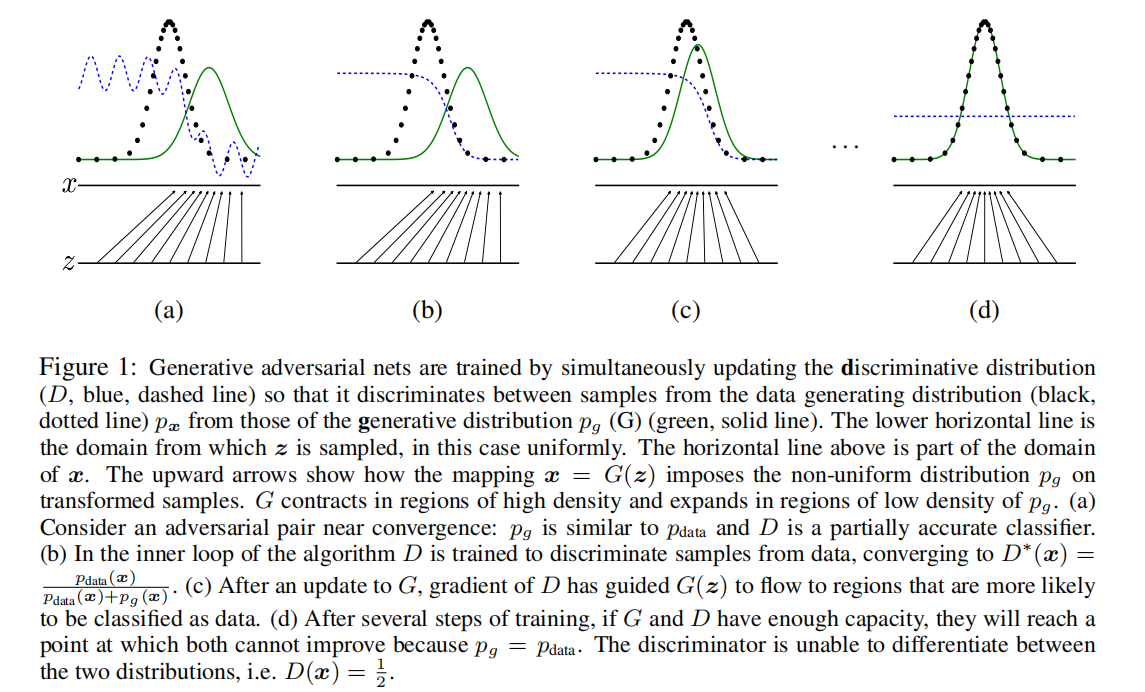
生成对抗网络
由两个网络组成,一个是生成模型用来产生样本,另一个是判别模型用来对样本进行判断。它们之间有一个对抗的关系。(一种竞争方式,来共同提升两者的能力)
生成器去学习一个关于 data  的分布,此处用
  表示,输入噪声表示为
  ,从噪
,从噪 ,其中的
,其中的  是一个可微的函数,本文采用的是一个多层感知机,
 表示感知机的参数。Discriminator 同样采用多层感知机构成,表示为
  ,它以 Generator 的输出以及真实 data 作为输入,产生一个 single scalar(也就是做一个分类判断,此处
  );
); 表示
表示  来自于真实 data 而不是
  的概率。我们将训练
  使得它能够最大限度地给 trainning examples 以及来自 的 samples 给出正确的 label(判断);与此同时,训练 使得
  最小化(等价于最大化
  ,也即是说
,也即是说  和真实 data 难以辨别)
In other words, D and G play the following two-player minimax game with value function V (G, D):
- 随机信号:信号任意时刻的值都是一个随机变量(即每次采样都是随机在样本分布中得到结果)。在随机信号分析(随机过程)过程中,不能采用简单的傅里叶变换。与之代替的是对随机信号的功率谱密度进行分析(对自相关函数进行傅里叶变换)。白噪声的功率谱密度函数是个常数,任意的随机信号可以看做是白噪声通过一个特定滤波器之后产生的结果。
- 为啥采用噪声的另一个原因:保证产生数据的随机性。
- 利用随机过程来理解样本更为合理。
- 为何采用期望?因为
本身就是随机变量,通常采用期望来作为评价指标。
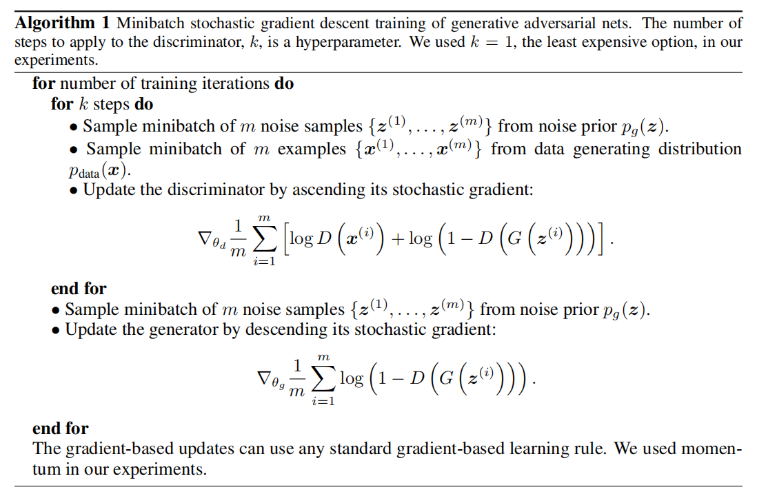
训练方面的指导
In practice, we must implement the game using an iterative, numerical approach. Optimizing D to completion in the inner loop of training is computationally prohibitive, and on finite datasets would result in overfifitting. Instead, we alternate between k steps of optimizing D and one step of optimizing G. This results in D being maintained near its optimal solution, so long as G changes slowly enough. This strategy is analogous to the way that SML/PCD [31, 29] training maintains samples from a Markov chain from one learning step to the next in order to avoid burning in a Markov chain as part of the inner loop of learning. The procedure is formally presented in Algorithm 1.
In practice, equation 1 may not provide suffificient gradient for G to learn well. Early in learning, when G is poor, D can reject samples with high confifidence because they are clearly different from the training data. In this case, log(1 − D(G(z))) saturates. Rather than training G to minimize log(1 − D(G(z))) we can train G to maximize log D(G(z)). This objective function results in the same fixed point of the dynamics of G and D but provides much stronger gradients early in learning.
理论结论
1、For G fifixed, the optimal discriminator D is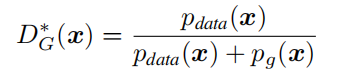
根据上面的结论,对优化目标(固定 G)进行重写有: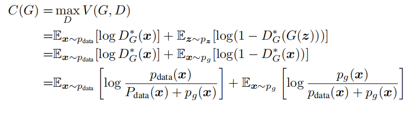
Theorem 1. The global minimum of the virtual training criterion C(G) is achieved if and only if  . At that point, C(G) achieves the value − _log 4._
优缺点分析
The disadvantages are primarily that there is no explicit representation of  , and that D must be synchronized well with G during training (in particular, G must not be trained too much without updating D, in order to avoid “the Helvetica scenario” in which G collapses too many values of z to the same value of x to have enough diversity to model pdata), much as the negative chains of a Boltzmann machine must be kept up to date between learning steps. The advantages are that Markov chains are never needed, only backprop is used to obtain gradients, no inference is needed during learning, and a wide variety of functions can be incorporated into the model. Table 2 summarizes the comparison of generative adversarial nets with other generative modeling approaches.
为何 GANs 能够取得非常不错的效果呢?因为 G 和 D 的训练都是一个循序渐进的过程。一开始给二者的任务是相对简单的,随着模型能够处理简单任务之后再对要求进行提高。这就像学数学一样,一上来就学微积分、矩阵论,再好的学生可能也会学不懂;我们应该从算术,方程等简单的知识开始。

若有收获,就点个赞吧
0 人点赞
