原文链接：Rich feature hierarchies for accurate object detection and semantic segmentation Author: Ross Girshick, Jeff Donahue, Trevor Darrell etc 博客学习：https://blog.csdn.net/briblue/article/details/82012575 https://zhuanlan.zhihu.com/p/30316608

Abstract

Our approach combines two key insights: (1) one can apply high-capacity convolutional neural networks (CNNs) to bottom-up region proposals in order to localize and segment objects and (2) when labeled training data is scarce(不足), supervised pre-training for an auxiliary task(辅助任务), followed by domain-specific fine-tuning, yields a significant performance boost.

Introduction

The last decade of progress on various visual recognition tasks has been based considerably on the use of SIFT and HOG.

SIFT: 一种特征提取的算法，其提取的特征具有：位置、尺度、旋转不变性； HOG: Histogram of Oriented Gradient, 同样是一种特征提取的方式；

Fukushima’s “neocognitron”, a biologicallyinspired hierarchical and shift-invariant model for pattern recognition, was an early attempt at just such a process. The neocognitron, however, lacked a supervised training algorithm. Building on Rumelhart et al. LeCun et al. showed that stochastic gradient descent via backpropagation was effective for training convolutional neural networks (CNNs), a class of models that extend the neocognitron.

This paper is the first to show that a CNN can lead to dramatically higher object detection performance on PASCAL VOC as compared to systems based on simpler HOG-like features. To achieve this result, we focused on two problems: localizing objects with a deep network and training a high-capacity model with only a small quantity of annotated detection data.
Unlike image classification, detection requires localizing (likely many) objects within an image. One approach frames localization as a regression problem. However, work from Szegedy et al. concurrent with our own, indicates that this strategy may not fare well in practice (they report a mAP of 30.5% on VOC 2007 compared to the 58.5% achieved by our method)

采用直接回归位置框，可能效果会差一些。（yolo就是采用回归的方式）

An alternative is to build a sliding-window detector. CNNs have been used in this way for at least two decades, typically on constrained object categories, such as faces and pedestrians.

滑动窗口的方式也可以用来检测目标，但是是比较老的方法了

We also considered adopting a sliding-window approach. However, units high up in our network, which has five convolutional layers, have very large receptive fields (195 × 195 pixels) and strides (32×32 pixels) in the input image, which makes precise localization within the sliding-window paradigm an open technical challenge.

如何理解这句话？网络层数高时，feature map 感受野很大，那么将其对应到滑动窗口时，将会出现滑动窗口偏大而导致定位不精确的情况发生。

Instead, we solve the CNN localization problem by operating within the “recognition using regions” paradigm, which has been successful for both object detection and semantic segmentation.
At test time, our method generates around 2000 category-independent region proposals for the input image, extracts a fixed-length feature vector from each proposal using a CNN, and then classifies each region with category-specific linear SVMs. We use a simple technique (affine image warping) to compute a fixed-size CNN input from each region proposal, regardless of the region’s shape. Figure 1 presents an overview of our method and highlights some of our results. Since our system combines region proposals with CNNs, we dub the method R-CNN: Regions with CNN features.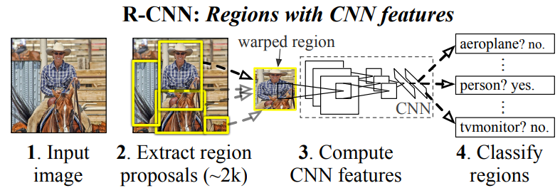

OverFeat uses a sliding-window CNN for detection and until now was the best performing method on ILSVRC2013 detection.

A second challenge faced in detection is that labeled data is scarce and the amount currently available is insufficient for training a large CNN. The conventional solution to this problem is to use unsupervised pre-training, followed by supervised fine-tuning.
The second principle contribution of this paper is to show that supervised pre-training on a large auxiliary dataset (ILSVRC), followed by domainspecific fine-tuning on a small dataset (PASCAL), is an effective paradigm for learning high-capacity CNNs when data is scarce.

这些表明了预训练模型的优点

Our system is also quite efficient. The only class-specific computations are a reasonably small matrix-vector product and greedy non-maximum suppression. This computational property follows from features that are shared across all categories and that are also two orders of magnitude lower dimensional than previously used region features.

Understanding the failure modes of our approach is also critical for improving it, and so we report results from the detection analysis tool of Hoiem et al. As an immediate consequence of this analysis, we demonstrate that a simple bounding-box regression method significantly reduces mislocalizations, which are the dominant error mode.

detection analysis tool? 边界框回归降低错误定位 — 这和前面的差别是什么？

Module design

Region proposals. A variety of recent papers offer methods for generating category-independent region proposals.

如何产生 Proposals 呢？

_Feature extraction. _We extract a 4096-dimensional feature vector from each region proposal using the Caffe implementation of the CNN described by Krizhevsky et al. Features are computed by forward propagating a mean-subtracted 227 × 227 RGB image through five convolutional layers and two fully connected layers.

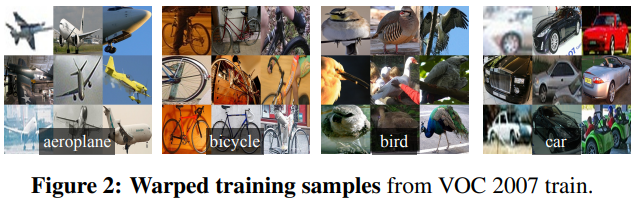
In order to compute features for a region proposal, we must first convert the image data in that region into a form that is compatible with the CNN (its architecture requires inputs of a fixed 227 × 227 pixel size). Of the many possible transformations of our arbitrary-shaped regions,_ we opt for the simplest. Regardless of the size or aspect ratio of the candidate region, we warp all pixels in a tight bounding box around it to the required size. _Prior to warping, we dilate the tight bounding box so that at the warped size there are exactly p pixels of warped image context around the original box (we use p = 16). Figure 2 shows a random sampling of warped training regions. Alternatives to warping are discussed in Appendix A.

为了使得对于 proposal regions 能够利用后面的CNN进行分析，文章采用了resize的方式处理图像，这样当然在很大程度上扭曲了原图。后面很大方法对此进行了改进。例如 ROI Pooling, ROI Align

Test-time detection

At test time, we run selective search on the test image to extract around 2000 region proposals (we use selective search’s “fast mode” in all experiments). We warp each proposal and forward propagate it through the CNN in order to compute features. Then, for each class, we score each extracted feature vector using the SVM trained for that class. Given all scored regions in an image, we apply a greedy non-maximum suppression (for each class independently) that rejects a region if it has an intersection-overunion (IoU) overlap with a higher scoring selected region larger than a learned threshold.

Training

Supervised pre-training. We discriminatively pre-trained the CNN on a large auxiliary dataset (ILSVRC2012 classification) using image-level annotations only (bounding-box labels are not available for this data). Pre-training was performed using the open source Caffe CNN library. In brief, our CNN nearly matches the performance of Krizhevsky et al. obtaining a top-1 error rate 2.2 percentage points higher on the ILSVRC2012 classification validation set. This discrepancy is due to simplifications in the training process.
Domain-specific fine-tuning.
Domain-specific fine-tuning. To adapt our CNN to the new task (detection) and the new domain (warped proposal windows), we continue stochastic gradient descent (SGD) training of the CNN parameters using only warped region proposals. Aside from replacing the CNN’s ImageNet specific 1000-way classification layer with a randomly initialized (N + 1)-way classification layer (where N is the number of object classes, plus 1 for background), the CNN architecture is unchanged. For VOC, N = 20 and for ILSVRC2013, N = 200. We treat all region proposals with ≥ 0.5 IoU overlap with a ground-truth box as positives for that box’s class and the rest as negatives. We start SGD at a learning rate of 0.001 (1/10th of the initial pre-training rate), which allows fine-tuning to make progress while not clobbering(破坏) the initialization. In each SGD iteration, we uniformly sample 32 positive windows (over all classes) and 96 background windows to construct a mini-batch of size 128. We bias the sampling towards positive windows because they are extremely rare compared to background.

前半段说的是预训练，后半段说的是微调，那么微调过程中那个 proposal 如何控制 positive 或者 negative 的呢？ => 事实上 proposals 的产生就相当于是构建一个模型训练数据集的过程。采用 selective search 等方法都可以产生 proposals，每张图产生的 proposals 是相同的，我们可以将其记录下来，对其打上标签，然后去训练后面的 CNN 网络（微调过程中还是用分类任务来训练网络，后面再去利用网络中间的 4096 维向量去训练一系列 SVMs）

Object category classifiers. _Consider training a binary classifier to detect cars. It’s clear that an image region tightly enclosing a car should be a positive example. Similarly, it’s clear that a background region, which has nothing to do with cars, should be a negative example. Less clear is how to label a region that partially overlaps a car. _We resolve this issue with an IoU overlap threshold, below which regions are defined as negatives. The overlap threshold, 0.3, was selected by a grid search over {0, 0.1, . . . , 0.5} on a validation set. We found that selecting this threshold carefully is important. Setting it to 0.5, as in [39], decreased mAP by 5 points. Similarly, setting it to 0 decreased mAP by 4 points. Positive examples are defined simply to be the ground-truth bounding boxes for each class.

Grid Search：一种调参手段；穷举搜索：在所有候选的参数选择中，通过循环遍历，尝试每一种可能性，表现最好的参数就是最终的结果。其原理就像是在数组里找最大值。（为什么叫网格搜索？以有两个参数的模型为例，参数a有3种可能，参数b有4种可能，把所有可能性列出来，可以表示成一个3*4的表格，其中每个cell就是一个网格，循环过程就像是在每个网格里遍历、搜索，所以叫 grid search）

Once features are extracted and training labels are applied, we optimize one linear SVM per class. Since the training data is too large to fit in memory, we adopt the standard hard negative mining method [17, 37]. Hard negative mining converges quickly and in practice mAP stops increasing after only a single pass over all images.

Results

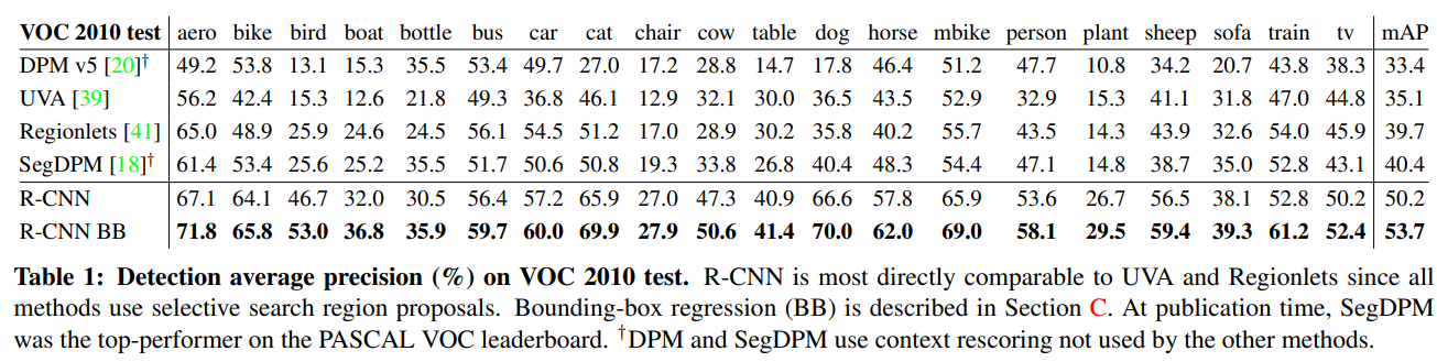
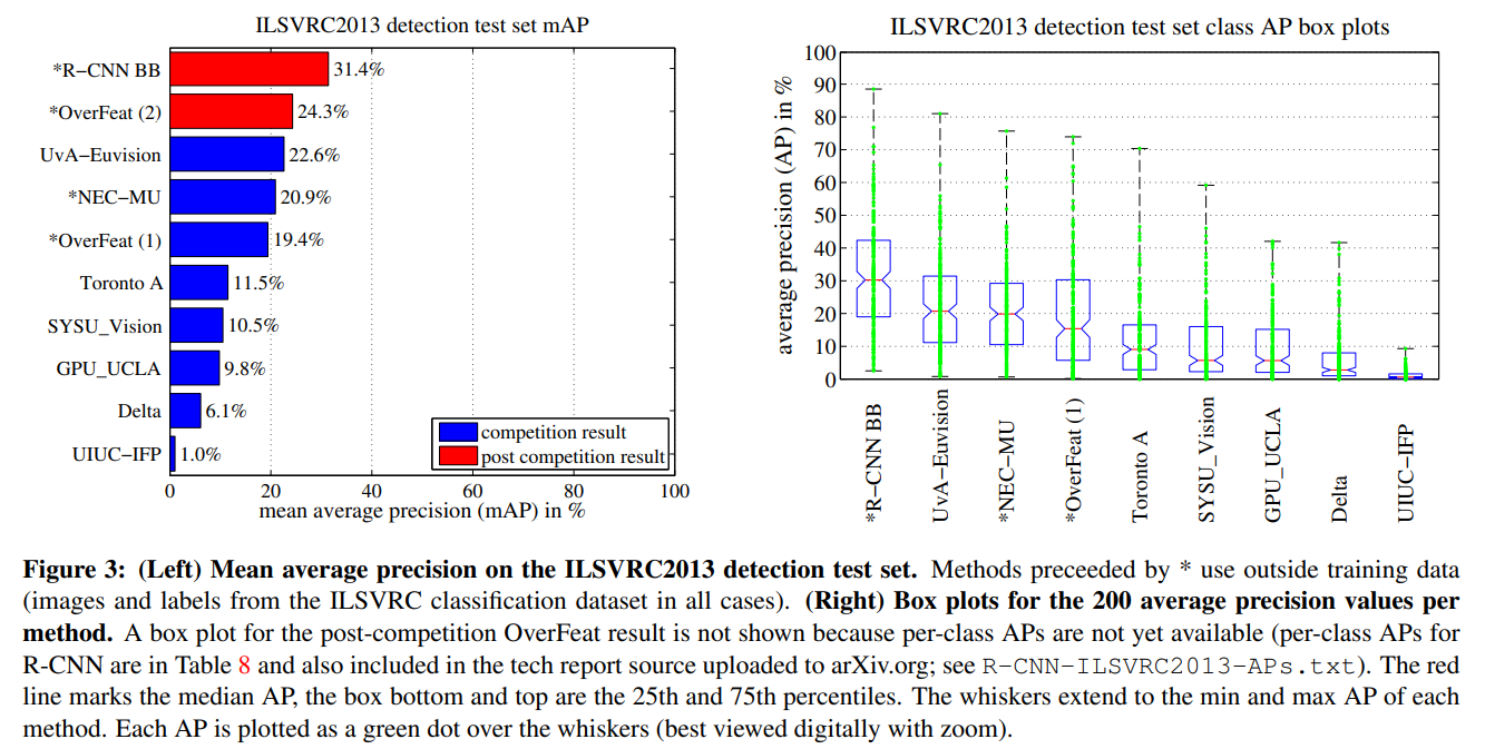
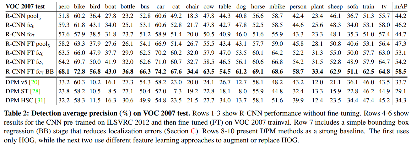
不同方法对比

R-CNN自己对比

可视化结果

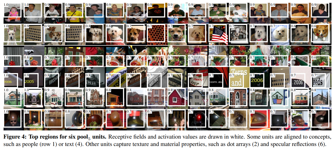
We visualize units from layer pool5 , which is the maxpooled output of the network’s fifth and final convolutional layer. The pool5 feature map is 6 × 6 × 256 = 9216-dimensional. Ignoring boundary effects, each pool5 unit has a receptive field of 195×195 pixels in the original 227×227 pixel input. A central pool5 unit has a nearly global view, while one near the edge has a smaller, clipped support.

从 layer pool5 映射到输入图片的 region proposals吗？

Each row in Figure 4 displays the top 16 activations for a pool5 unit from a CNN that we fine-tuned on VOC 2007 trainval. Six of the 256 functionally unique units are visualized (Appendix D includes more). These units were selected to show a representative sample of what the network learns. In the second row, we see a unit that fires on dog faces and dot arrays. The unit corresponding to the third row is a red blob detector. There are also detectors for human faces and more abstract patterns such as text and triangular structures with windows. The network appears to learn a representation that combines a small number of class-tuned features together with a distributed representation of shape, texture, color, and material properties. The subsequent fully connected layer fc6 has the ability to model a large set of compositions of these rich features.

Ablation studies

Performance layer-by-layer, without fine-tuning. To understand which layers are critical for detection performance, we analyzed results on the VOC 2007 dataset for each of the CNN’s last three layers. Layer pool5 was briefly described in Section 3.1. The final two layers are summarized below.

Layer fc6 is fully connected to pool5 . To compute features, it multiplies a weight matrix by the pool5 feature map (reshaped as a 9216-dimensional vector) and then adds a vector of biases. This intermediate vector is component-wise half-wave rectified ().

Layer fc7 is the final layer of the network. It is implemented by multiplying the features computed by fc6 by a 4096 × 4096 weight matrix, and similarly adding a vector of biases and applying half-wave rectification.

从表2 看来倒是挺奇怪的：Analyzing performance layer-by-layer (Table 2 rows 1-3) reveals that features from fc7 generalize worse than features from fc6. This means that 29%, or about 16.8 million, of the CNN’s parameters can be removed without degrading mAP. More surprising is that removing both fc7 and fc6 produces quite good results even though pool5 features are computed using only 6% of the CNN’s parameters. Much of the CNN’s representational power comes from its convolutional layers, rather than from the much larger densely connected layers. This finding suggests potential utility in computing a dense feature map, in the sense of HOG, of an arbitrary-sized image by using only the convolutional layers of the CNN. This representation would enable experimentation with sliding-window detectors, including DPM, on top of pool5 features.

全连接层对提升效果没有多大作用。

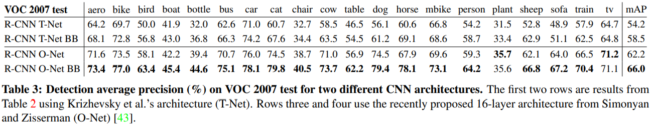
Network architectures

下面是采用不同网络得到的效果，其中 O-Net 即 OxfordNet，T-Net 即 TorontoNet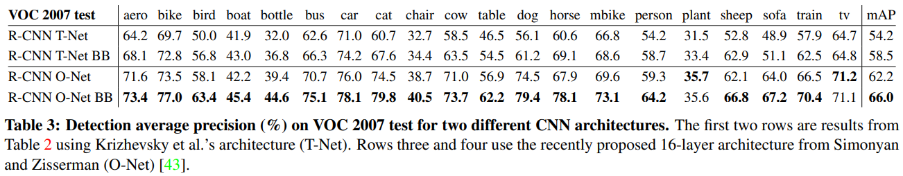

Bounding-box regression

Based on the error analysis, we implemented a simple method to reduce localization errors. Inspired by the bounding-box regression employed in DPM, we train a linear regression model to predict a new detection window given the pool5 features for a selective search region proposal. Full details are given in Appendix C. Results in Table 1, Table 2, and Figure 5 show that this simple approach fixes a large number of mislocalized detections, boosting mAP by 3 to 4 points.

与 yolo 回归很类似，是在 region proposals 和 CNN features 的基础上回归 BB 的。 模型的公式表达：为何有效？没看明白（如何建模？） https://zhuanlan.zhihu.com/p/30316608

Dataset overview

The ILSVRC2013 detection dataset is split into three sets: train (395,918), val (20,121), and test (40,152), where the number of images in each set is in parentheses. The val and test splits are drawn from the same image distribution. These images are scene-like and similar in complexity (number of objects, amount of clutter, pose variability, etc.) _to PASCAL VOC images. The val and test splits are exhaustively annotated, meaning that in each image all instances from all 200 classes are labeled with bounding boxes. The train set, in contrast, is drawn from the ILSVRC2013 classification image distribution. These images have more variable complexity with a skew towards images of a single centered object. Unlike val and test, the train images (due to their large number) are not exhaustively annotated(说的是一张图片可能只标注了一个对象). In any given train image, instances from the 200 classes may or may not be labeled. In addition to these image sets, each class has an extra set of negative images. Negative images are manually checked to validate that they do not contain any instances of their associated class. _The negative image sets were not used in this work. More information on how ILSVRC was collected and annotated can be found in [11, 36].

The nature of these splits presents a number of choices for training R-CNN. The train images cannot be used for hard negative mining, because annotations are not exhaustive. Where should negative examples come from? Also, the train images have different statistics than val and test. Should the train images be used at all, and if so, to what extent? While we have not thoroughly evaluated a large number of choices, we present what seemed like the most obvious path based on previous experience.

Our general strategy is to rely heavily on the val set and use some of the train images as an auxiliary source of positive examples. To use val for both training and validation, we split it into roughly equally sized “val1” and “val2” sets. Since some classes have very few examples in val (the smallest has only 31 and half have fewer than 110), it is important to produce an approximately class-balanced partition. To do this, a large number of candidate splits were generated and the one with the smallest maximum relative class imbalance was selected. Each candidate split was generated by clustering val images using their class counts as features, followed by a randomized local search that may improve the split balance. The particular split used here has a maximum relative imbalance of about 11% and a median relative imbalance of 4%. The val1/val2 split and code used to produce them will be publicly available to allow other researchers to compare their methods on the val splits used in this report.

没看懂在干嘛… 这个数据处理，分配等问题，看起来超级麻烦的…

Region proposals

We followed the same region proposal approach that was used for detection on PASCAL. Selective search was run in “fast mode” on each image in val1, val2, and test (but not on images in train). One minor modification was required to deal with the fact that selective search is not scale invariant and so the number of regions produced depends on the image resolution. ILSVRC image sizes range from very small to a few that are several mega-pixels, and so we resized each image to a fixed width (500 pixels) before running selective search. On val, selective search resulted in an average of 2403 region proposals per image with a 91.6% recall of all ground-truth bounding boxes (at 0.5 IoU threshold). This recall is notably lower than in PASCAL, where it is approximately 98%, indicating significant room for improvement in the region proposal stage.

实验还考虑了不同数据集的冗余问题。

Training data

For training data, we formed a set of images and boxes that includes all selective search and ground-truth boxes from val1 together with up to N ground-truth boxes per class from train (if a class has fewer than N ground-truth boxes in train, then we take all of them). We’ll call this dataset of images and boxes val1+trainN . In an ablation study, we show mAP on val2 for N ∈ {0, 500, 1000} (Section 4.5).

For SVM training, all ground-truth boxes from val1+trainN were used as positive examples for their respective classes. Hard negative mining was performed on a randomly selected subset of 5000 images from val1. An initial experiment indicated that mining negatives from all of val1, versus a 5000 image subset (roughly half of it), resulted in only a 0.5 percentage point drop in mAP, while cutting SVM training time in half. No negative examples were taken from train because the annotations are not exhaustive. The extra sets of verified negative images were not used. The bounding-box regressors were trained on val1.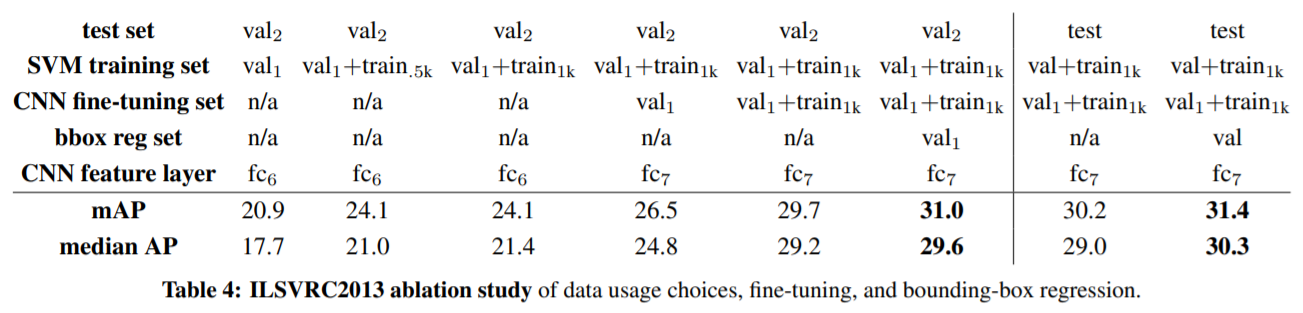

部分总结

• 文章在数据处理方面提出了一些指导性意见；
• 在预训练方面做了一些研究；
• 在网络选择方面展示了一些选择的过程；
• 基于 region proposals 的坐标回归；

方法核心：

• region proposals：selective search
• region proposals 的 resize 以适应后面的 CNN；
• BBox 的预测：借助 CNN 提取的特征
• CNN 的分类：SVM 分类器