分形图形一般都有自相似性,这就是说如果将分形图形的局部不断放大并进行观察,将发现精细的结构,如果再放大,就会再度出现更精细的结构,可谓层出不穷,永无止境。
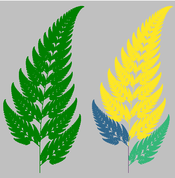
import numpy as npimport matplotlib.pyplot as plt# 蕨类植物叶子的迭代函数和其概率值eq1 = np.array([[0, 0, 0], [0, 0.16, 0]])p1 = 0.01eq2 = np.array([[0.2, -0.26, 0], [0.23, 0.22, 1.6]])p2 = 0.07eq3 = np.array([[-0.15, 0.28, 0], [0.26, 0.24, 0.44]])p3 = 0.07eq4 = np.array([[0.85, 0.04, 0], [-0.04, 0.85, 1.6]])p4 = 0.85def ifs(p, eq, init, n):"""进行函数迭代p: 每个函数的选择概率列表eq: 迭代函数列表init: 迭代初始点n: 迭代次数返回值:每次迭代所得的X坐标数组, Y坐标数组, 计算所用的函数下标"""# 迭代向量的初始化pos = np.ones(3, dtype=np.float)pos[:2] = init# 通过函数概率,计算函数的选择序列p = np.add.accumulate(p)rands = np.random.rand(n)select = np.ones(n, dtype=np.int) * (n - 1)for i, x in enumerate(p[::-1]):select[rands < x] = len(p) - i - 1# 结果的初始化result = np.zeros((n, 2), dtype=np.float)c = np.zeros(n, dtype=np.float)for i in range(n):eqidx = select[i] # 所选的函数下标tmp = np.dot(eq[eqidx], pos) # 进行迭代pos[:2] = tmp # 更新迭代向量# 保存结果result[i] = tmpc[i] = eqidxreturn result[:, 0], result[:, 1], cx, y, c = ifs([p1, p2, p3, p4], [eq1, eq2, eq3, eq4], [0, 0], 1000000)plt.figure(figsize=(6, 6))plt.subplot(121)plt.scatter(x, y, s=1, c="g", marker="s", linewidths=0)plt.axis("equal")plt.axis("off")plt.subplot(122)plt.scatter(x, y, s=1, c=c, marker="s", linewidths=0)plt.axis("equal")plt.axis("off")plt.subplots_adjust(left=0, right=1, bottom=0, top=1, wspace=0, hspace=0)plt.gcf().patch.set_facecolor("silver")plt.show()

若有收获,就点个赞吧
0 人点赞
