在本教程中,我们将学习Seurat3中使用
SCTransform方法对单细胞测序数据进行标准化处理的方法。该方法是Seurat3中新引入的数据标准化方法,可以代替之前NormalizeData,ScaleData, 和FindVariableFeatures依次运行的三个命令,可以有效的去除一些技术误差和批次效应。
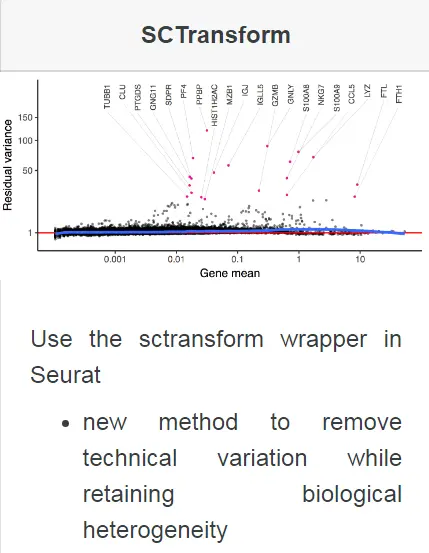
Apply sctransform normalization:
- Note that this single command replaces
NormalizeData,ScaleData, andFindVariableFeatures.- Transformed data will be available in the
SCT assay, which is set as the default after running sctransform- During normalization, we can also
remove confounding sources of variation, for example, mitochondrial mapping percentage
其详细的方法原理可以查看19年发表在GB上的这篇文章Normalization and variance stabilization of single-cell RNA-seq data using regularized negative binomial regression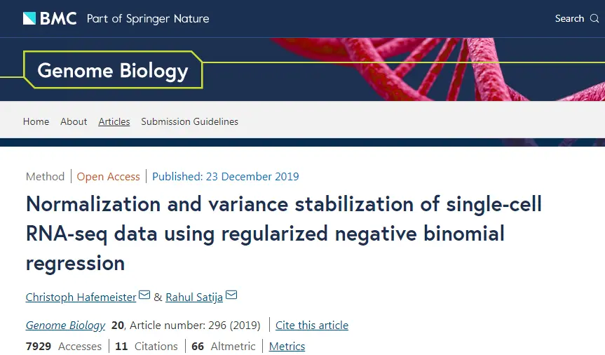
安装并加载所需的R包
#install.packages("Seurat")library(Seurat)library(ggplot2)library(sctransform)
加载数据构建Seurat对象
pbmc_data <- Read10X(data.dir = "/home/dongwei/data/pbmc3k/filtered_gene_bc_matrices/hg19/")pbmc <- CreateSeuratObject(counts = pbmc_data)View(pbmc)
使用SCTransform进行数据标准化
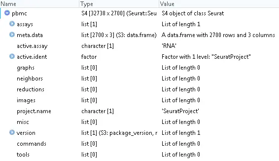
# store mitochondrial percentage in object meta data# 计算每个细胞中的线粒体含量pbmc <- PercentageFeatureSet(pbmc, pattern = "^MT-", col.name = "percent.mt")# run sctransform# 使用vars.to.regress参数指定对线粒体含量进行校正pbmc <- SCTransform(pbmc, vars.to.regress = "percent.mt", verbose = FALSE)pbmcAn object of class Seurat45310 features across 2700 samples within 2 assaysActive assay: SCT (12572 features, 3000 variable features)1 other assay present: RNA
可以看到,执行完SCTranform标准化后会生成一个新的SCT Assay,里面存储着标准化后的一些数据信息。
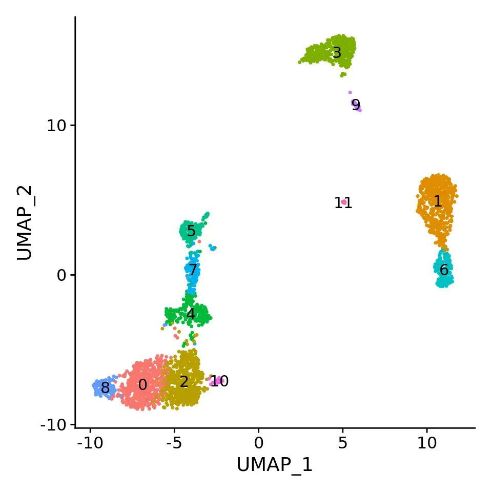
数据降维、聚类与可视化
# These are now standard steps in the Seurat workflow for visualization and clusteringpbmc <- RunPCA(pbmc, verbose = FALSE)pbmc <- RunUMAP(pbmc, dims = 1:30, verbose = FALSE)pbmc <- FindNeighbors(pbmc, dims = 1:30, verbose = FALSE)pbmc <- FindClusters(pbmc, verbose = FALSE)DimPlot(pbmc, label = TRUE) + NoLegend()
为什么我们在使用sctransform标准化后选择更多PC?
- 在常规的数据标准化过程中,我们在进行PCA降维后选择了10个PC用于后续的聚类分析,使用少量的PC既能捕捉到主要的生物学差异,又不会引入更多的技术差异。而在SCTransform标准化过程中,我们在PCA降维后选择了30个PC用于后续的聚类分析,这是因为sctransform标准化过程执行了更有效的规范化,从而可以更强烈的消除数据中的技术影响。有趣的是,我们发现在使用sctransform时,通常可以设置较高的参数获得理想的结果。
- 在常规的数据标准化过程中,即使经过了标准的对数归一化处理,测序深度的变化仍然是一个混杂因素,并且这种影响可能会微妙地影响更高的PC。而在sctransform中,此效果已大大减轻,这意味着更高的PC更可能代表那些微妙的但与生物学相关的异质性来源,因此可能会改善下游的聚类分析。
- 此外,常规分析中FindVariableFeatures默认会得到2000个高变异基因(HVGs),而使用sctransform进行标准化时,因为使用了更多的PCs,算法也更加优化,所以默认会得到3000个HVGs。sctransform认为:新增加的这1000个基因就包含了之前没有检测到的微弱的生物学差异。而且,即使使用全部的基因去做下游分析,得到的结果也是和sctransform这3000个基因的结果相似。
执行sctransform标准化后的数据存储在哪里?
- pbmc[[“SCT”]]@scale.data :存储了残差数据(归一化值),并直接用作PCA的输入。这个数据不是稀疏矩阵,因此会占用大量内存。不过SCTransform函数计算的时候,为了节省内存,默认使用了return.only.var.genes = TRUE ,只保留差异基因的结果。
- pbmc[[“SCT”]]@counts :存储了校正后的UMI count值。
- pbmc[[“SCT”]]@data:存储了校正后count值的log-normalized结果,有利于后面的可视化。
当然,我们还可以使用管道符将上述步骤连接在一起,使用单行代码实现分析
pbmc <- CreateSeuratObject(pbmc_data) %>%PercentageFeatureSet(pattern = "^MT-", col.name = "percent.mt") %>%SCTransform(vars.to.regress = "percent.mt") %>% RunPCA() %>%FindNeighbors(dims = 1:30) %>%RunUMAP(dims = 1:30) %>%FindClusters()
使用marker基因对细胞分群进行注释和可视化
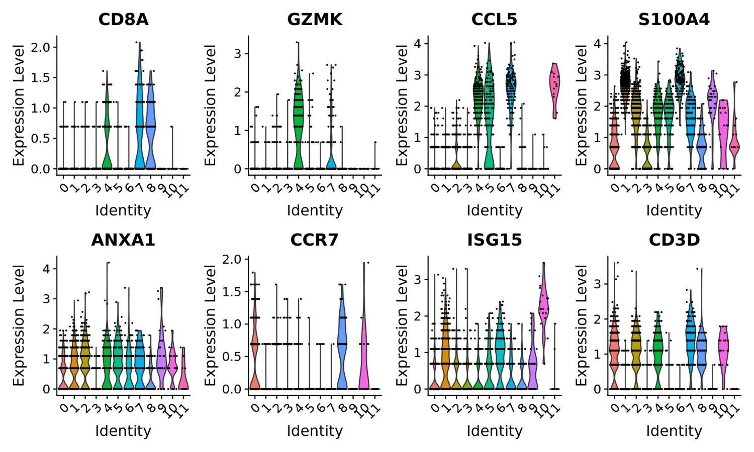
- Clear separation of at least 3
CD8 T cellpopulations (naive, memory, effector), based onCD8A, GZMK, CCL5, GZMKexpression- Clear separation of three
CD4 T cellpopulations (naive, memory, IFN-activated) based onS100A4, CCR7, IL32, and ISG15- Additional developmental sub-structure in
B cellcluster, based onTCL1A, FCER2- Additional separation of
NK cellsinto CD56dim vs. bright clusters, based onXCL1 and FCGR3A
# These are now standard steps in the Seurat workflow for visualization and clustering Visualize# canonical marker genes as violin plots.VlnPlot(pbmc, features = c("CD8A", "GZMK", "CCL5", "S100A4", "ANXA1", "CCR7", "ISG15", "CD3D"), pt.size = 0.2, ncol = 4)
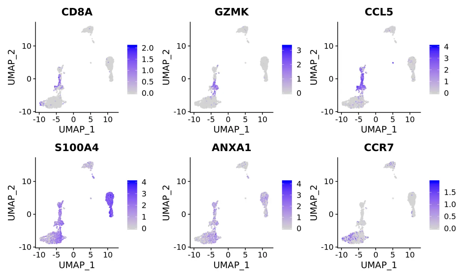
# Visualize canonical marker genes on the sctransform embedding.FeaturePlot(pbmc, features = c("CD8A", "GZMK", "CCL5", "S100A4", "ANXA1", "CCR7"), pt.size = 0.2, ncol = 3)
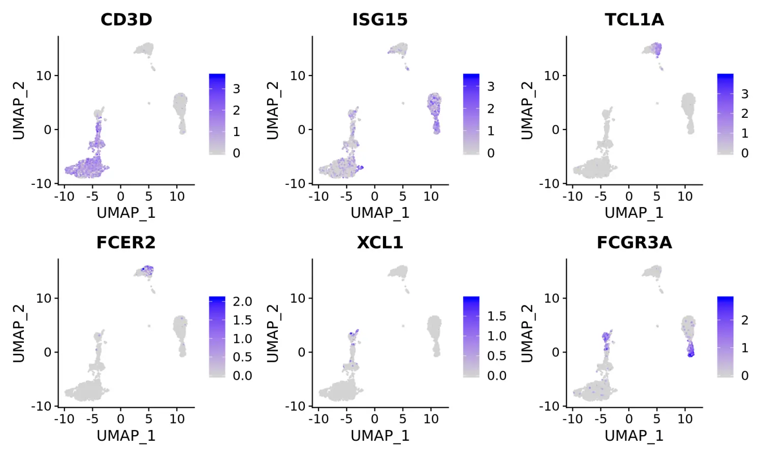
FeaturePlot(pbmc, features = c("CD3D", "ISG15", "TCL1A", "FCER2", "XCL1", "FCGR3A"), pt.size = 0.2, ncol = 3)
参考来源:https://satijalab.org/seurat/v3.1/sctransform_vignette.html

若有收获,就点个赞吧
0 人点赞
