使用Signac包进行单细胞ATAC-seq数据分析（三）：scATAC-seq data integration

在本教程中，我们将学习使用Signac包对多样本的scATAC-seq数据进行整合分析。这里，我们对来自10x Genomics和sci-ATAC-seq技术测序的成年小鼠大脑的多个单细胞ATAC-seq数据集进行了整合分析。

其中，10x Genomics平台产生的原始数据可从官网下载：

• The Raw data
• The Metadata
• The fragments file
• The fragments file index

sci-ATAC-seq技术产生的数据集由Cusanovich和Hill等人生成。原始数据可从作者的网站下载：

• Cell metadata
• Count matrix

我们将演示使用Seurat v3中的数据整合方法（dataset integration and label transfer）对多个scATAC-seq数据集进行整合分析，以及使用harmony包进行数据整合。

安装并加载所需的R包

if (!requireNamespace("BiocManager", quietly = TRUE))
    install.packages("BiocManager")
BiocManager::install("rtracklayer")
library(devtools)
install_github("immunogenomics/harmony")
library(Signac)
library(Seurat)
library(patchwork)
set.seed(1234)

加载数据集并构建Seurat对象

# this object was created following the mouse brain vignette
# 加载10x Genomics的小鼠大脑的scATAC-seq数据
tenx <- readRDS(file = "/home/dongwei/scATAC-seq/brain/10x/adult_mouse_brain.rds")
tenx$tech <- '10x'
tenx$celltype <- Idents(tenx)
# 加载sci-ATAC-seq的小鼠大脑数据
sci.metadata <- read.table(
  file = "/home/dongwei/scATAC-seq/brain/sci/cell_metadata.txt",
  header = TRUE,
  row.names = 1,
  sep = "\t"
)
# subset to include only the brain data
sci.metadata <- sci.metadata[sci.metadata$tissue == 'PreFrontalCortex', ]
sci.counts <- readRDS(file = "/home/dongwei/scATAC-seq/brain/sci/atac_matrix.binary.qc_filtered.rds")
sci.counts <- sci.counts[, rownames(x = sci.metadata)]

数据预处理

在上述两个数据集中，sci-ATAC-seq数据是比对到小鼠mm9参考基因组的，而10x的数据是比对到小鼠mm10参考基因组的，因此这两个数据集中peaks的基因组坐标信息是不同的。我们可以使用rtracklayer包将mm9参考基因组的坐标信息转换到mm10中，并使用mm10的坐标更换sci-ATAC-seq数据中peaks的坐标，其中liftover转换的chain文件可以从UCSC官网进行下载。

# 将peaks坐标信息转换成GRanges格式
sci_peaks_mm9 <- StringToGRanges(regions = rownames(sci.counts), sep = c("_", "_"))
# 导入mm9ToMm10.over.chain文件
mm9_mm10 <- rtracklayer::import.chain("/home/dongwei/data/liftover/mm9ToMm10.over.chain")
# 使用rtracklayer包中的liftOver函数转换坐标信息
sci_peaks_mm10 <- rtracklayer::liftOver(x = sci_peaks_mm9, chain = mm9_mm10)
names(sci_peaks_mm10) <- rownames(sci.counts)
# discard any peaks that were mapped to >1 region in mm10
correspondence <- S4Vectors::elementNROWS(sci_peaks_mm10)
sci_peaks_mm10 <- sci_peaks_mm10[correspondence == 1]
sci_peaks_mm10 <- unlist(sci_peaks_mm10)
sci.counts <- sci.counts[names(sci_peaks_mm10), ]
# rename peaks with mm10 coordinates
rownames(sci.counts) <- GRangesToString(grange = sci_peaks_mm10)
# create Seurat object and perform some basic QC filtering
# 构建Seurat对象
sci <- CreateSeuratObject(
  counts = sci.counts,
  meta.data = sci.metadata,
  assay = 'peaks',
  project = 'sci'
)
# 数据过滤
sci.ds <- sci[, sci$nFeature_peaks > 2000 & sci$nCount_peaks > 5000 & !(sci$cell_label %in% c("Collisions", "Unknown"))]
sci$tech <- 'sciATAC'
# 使用RunTFIDF函数进行数据归一化
sci <- RunTFIDF(sci)
# 使用FindTopFeatures函数提取高变异的peaks
sci <- FindTopFeatures(sci, min.cutoff = 50)
# 使用RunSVD函数进行线性降维
sci <- RunSVD(sci, n = 30, reduction.name = 'lsi', reduction.key = 'LSI_')
# 使用RunUMAP函数进行非线性降维
sci <- RunUMAP(sci, reduction = 'lsi', dims = 2:30)

现在，我们构建好了两个scATAC-seq对象，并且它们都含有基于相同的mm10参考基因组坐标系统得到的peaks信息。但是，由于这两个实验都单独进行了peak calling，因此这两个数据集中得到的peaks坐标不太可能完全重叠。为了在我们要整合的数据集中具有共同的特征，我们可以基于10x Genomics数据集对sci-ATAC-seq中peaks的reads进行计数，并使用这些计数创建一个新的assay。

# find peaks that intersect in both datasets
# 使用GetIntersectingFeatures函数提取两个数据集中重叠的peak区域
intersecting.regions <- GetIntersectingFeatures(
  object.1 = sci,
  object.2 = tenx,
  sep.1 = c("-", "-"),
  sep.2 = c(":", "-")
)
# choose a subset of intersecting peaks
peaks.use <- sample(intersecting.regions[[1]], size = 10000, replace = FALSE)
# count fragments per cell overlapping the set of peaks in the 10x data
# 使用FeatureMatrix函数对peaks中的reads进行计数
sci_peaks_tenx <- FeatureMatrix(
  fragments = GetFragments(object = tenx, assay = 'peaks'),
  features = StringToGRanges(peaks.use),
  cells = colnames(tenx)
)
# create a new assay and add it to the 10x dataset
# 使用CreateAssayObject函数新建一个assay对象
tenx[['sciPeaks']] <- CreateAssayObject(counts = sci_peaks_tenx, min.cells = 1)
# 数据归一化
tenx <- RunTFIDF(object = tenx, assay = 'sciPeaks')

多样本scATAC-seq数据集的整合

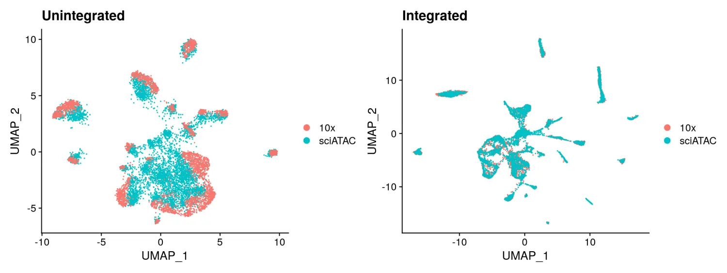
在进行数据整合之前，我们最好先检查下是否存在数据集特异的差异，并将其删除。如果没有，我们可以简单地将多个对象进行合并而不执行整合。在本示例中，由于使用不同的测序技术，两个数据集之间存在很大的差异。我们可以使用Seurat v3中的数据整合方法来消除这种影响。

# 先简单的将两个数据集进行合并看一下聚类的效果
# Look at the data without integration first
# 使用MergeWithRegions函数将两个数据对象进行合并
unintegrated <- MergeWithRegions(
  object.1 = sci,
  object.2 = tenx,
  assay.1 = 'peaks',
  assay.2 = 'sciPeaks',
  sep.1 = c("-", "-"),
  sep.2 = c("-", "-")
)
# 对合并后数据进行归一化，特征选择和降维可视化
unintegrated <- RunTFIDF(unintegrated)
unintegrated <- FindTopFeatures(unintegrated, min.cutoff = 50)
unintegrated <- RunSVD(unintegrated, n = 30, reduction.name = 'lsi', reduction.key = 'LSI_')
unintegrated <- RunUMAP(unintegrated, reduction = 'lsi', dims = 2:30)
p1 <- DimPlot(unintegrated, group.by = 'tech', pt.size = 0.1) + ggplot2::ggtitle("Unintegrated")
# 使用Seurat v3的数据整合方法进行数据集的整合
# find integration anchors between 10x and sci-ATAC
# 使用FindIntegrationAnchors函数识别共享的整合anchors
anchors <- FindIntegrationAnchors(
  object.list = list(tenx, sci),
  anchor.features = peaks.use,
  assay = c('sciPeaks', 'peaks'),
  k.filter = NA
)
# integrate data and create a new merged object
# 使用IntegrateData函数根据识别的anchors进行数据整合
integrated <- IntegrateData(
  anchorset = anchors,
  weight.reduction = sci[['lsi']],
  dims = 2:30,
  preserve.order = TRUE
)
# we now have a "corrected" TF-IDF matrix, and can run LSI again on this corrected matrix
# 对整合后的数据进行降维可视化
integrated <- RunSVD(
  object = integrated,
  n = 30,
  reduction.name = 'integratedLSI'
)
integrated <- RunUMAP(
  object = integrated,
  dims = 2:30,
  reduction = 'integratedLSI'
)
p2 <- DimPlot(integrated, group.by = 'tech', pt.size = 0.1) + ggplot2::ggtitle("Integrated")
p1 + p2

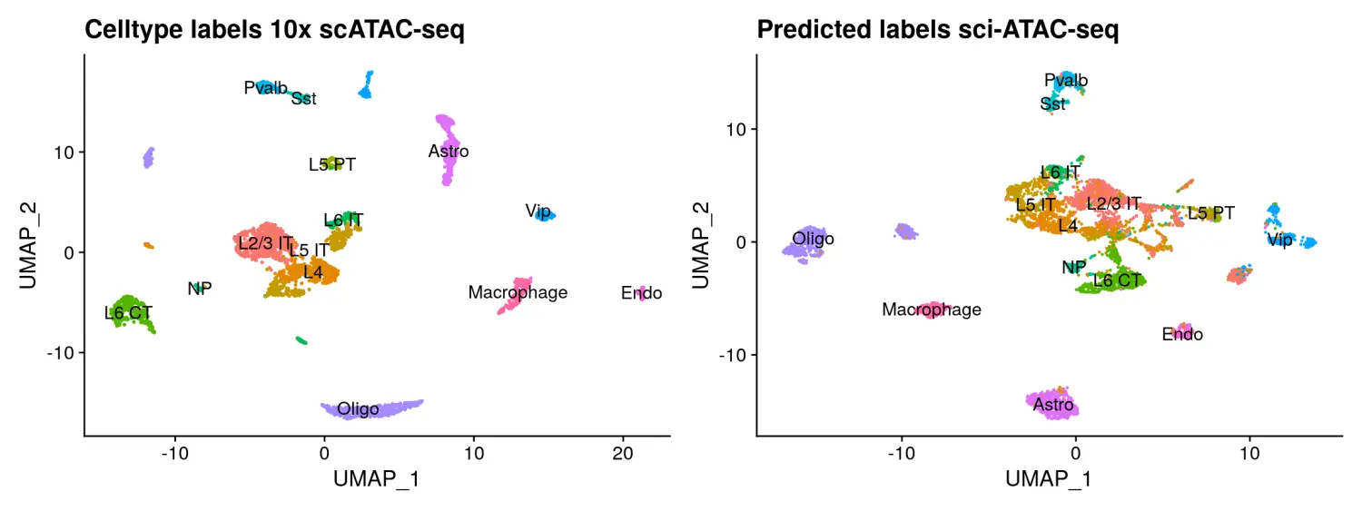
Label transfer

我们还可以使用Seurat v3中的Label transfer方法进行数据集的整合，它将数据从一个query数据集映射到另一个reference数据集中。在这里，我们通过将细胞类型标签从10x Genomics scATAC-seq数据映射到到sci-ATAC-seq数据中。

# 使用FindTransferAnchors函数识别整合的anchors
transfer.anchors <- FindTransferAnchors(
  reference = tenx,
  query = sci,
  reference.assay = 'sciPeaks',
  query.assay = 'peaks',
  reduction = 'cca',
  features = peaks.use,
  k.filter = NA
)
# 使用TransferData函数基于识别好的anchors进行数据映射整合
predicted.id <- TransferData(
  anchorset = transfer.anchors,
  refdata = tenx$celltype,
  weight.reduction = sci[['lsi']],
  dims = 2:30
)
sci <- AddMetaData(
  object = sci,
  metadata = predicted.id
)
sci$predicted.id <- factor(sci$predicted.id, levels = levels(tenx$celltype))  # to make the colors match
# 数据可视化
p3 <- DimPlot(tenx, group.by = 'celltype', label = TRUE) + NoLegend() + ggplot2::ggtitle("Celltype labels 10x scATAC-seq")
p4 <- DimPlot(sci, group.by = 'predicted.id', label = TRUE) + NoLegend() + ggplot2::ggtitle("Predicted labels sci-ATAC-seq")
p3 + p4

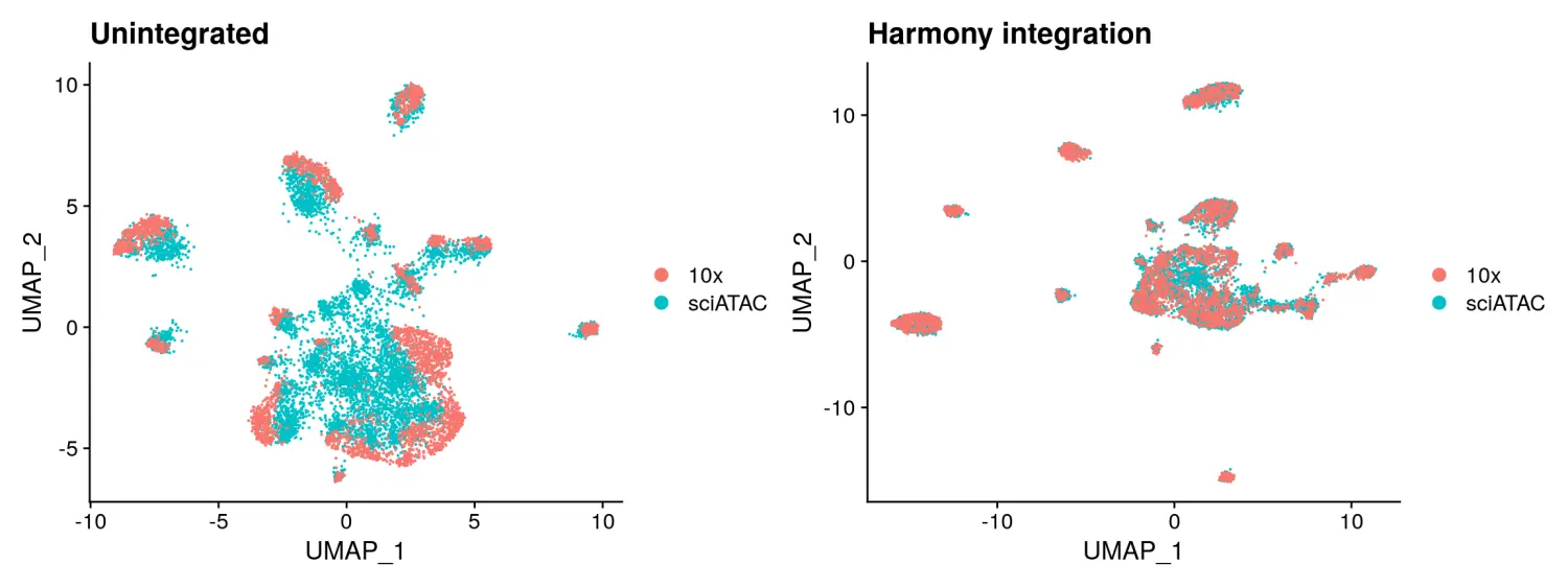
Integration with Harmony 使用Harmony包进行数据整合

Harmony需要一个对象作为输入，因此这里我们使用MergeWithRegions函数以coordinate-aware的方式将sci-ATAC-seq数据集和10x的scATAC-seq数据集进行合并，然后对合并后的对象进行LSI线性降维。数据降维后，我们可以使用RunHarmony函数调用Harmony的方法进行数据的整合，并提供用作分组变量的技术来消除sci-ATAC-seq和10x Genomics scATAC-seq数据集之间的批次差异。这会产生一组“校正”的LSI嵌入，可以进一步用于UMAP或tSNE降维，并进行细胞聚类分群。

# 加载harmony包
library(harmony)
# 使用RunHarmony函数进行数据整合
hm.integrated <- RunHarmony(
  object = unintegrated,
  group.by.vars = 'tech',
  reduction = 'lsi',
  assay.use = 'peaks',
  project.dim = FALSE
)
# re-compute the UMAP using corrected LSI embeddings
# 数据降维可视化
hm.integrated <- RunUMAP(hm.integrated, dims = 2:30, reduction = 'harmony')
p5 <- DimPlot(hm.integrated, group.by = 'tech', pt.size = 0.1) + ggplot2::ggtitle("Harmony integration")
p1 + p5

参考来源：https://satijalab.org/signac/articles/integration.html