在本教程中,我们将学习使用Seurat3分析和探索多模式数据。尽管这是一个初始版本,但我们很高兴在将来为多模式数据集的分析发布重要的新功能。
在这里,我们分析了由
CITE-seq产生的8,617个脐带血单核细胞(CBMC)的数据集。在该数据集中,我们同时测量了单细胞转录组和11种表面蛋白的表达,并用DNA条形码抗体对蛋白的表达水平进行了定量。
加载所需的R包和数据集
# Load in the RNA UMI matrix# Note that this dataset also contains ~5% of mouse cells, which we can use as negative controls for the protein measurements. For this reason, the gene expression matrix has HUMAN_ or MOUSE_appended to the beginning of each gene.# 读取基因表达矩阵cbmc.rna <- as.sparse(read.csv(file = "../data/GSE100866_CBMC_8K_13AB_10X-RNA_umi.csv.gz", sep = ",", header = TRUE, row.names = 1))# To make life a bit easier going forward, we're going to discard all but the top 100 most highly expressed mouse genes, and remove the 'HUMAN_' from the CITE-seq prefixcbmc.rna <- CollapseSpeciesExpressionMatrix(cbmc.rna)# Load in the ADT UMI matrix# 读取ADT UMI矩阵cbmc.adt <- as.sparse(read.csv(file = "../data/GSE100866_CBMC_8K_13AB_10X-ADT_umi.csv.gz", sep = ",", header = TRUE, row.names = 1))# When adding multimodal data to Seurat, it's okay to have duplicate feature names. Each set of modal data (eg. RNA, ADT, etc.) is stored in its own Assay object. One of these Assay objects is called the 'default assay', meaning it's used for all analyses and visualization. To pull data from an assay that isn't the default, you can specify a key that's linked to an assay for feature pulling. To see all keys for all objects, use the Key function. Lastly, we observed poor enrichments for CCR5, CCR7, and CD10 - and therefore remove them from the matrix# (optional)cbmc.adt <- cbmc.adt[setdiff(rownames(x = cbmc.adt), c("CCR5", "CCR7", "CD10")), ]
构建Seurat对象,并根据基因表达进行聚类
# 创建Seurat对象cbmc <- CreateSeuratObject(counts = cbmc.rna)# 数据标准化# standard log-normalizationcbmc <- NormalizeData(cbmc)# choose ~1k variable featurescbmc <- FindVariableFeatures(cbmc)# standard scaling (no regression)cbmc <- ScaleData(cbmc)# PCA降维# Run PCA, select 13 PCs for tSNE visualization and graph-based clusteringcbmc <- RunPCA(cbmc, verbose = FALSE)ElbowPlot(cbmc, ndims = 50)
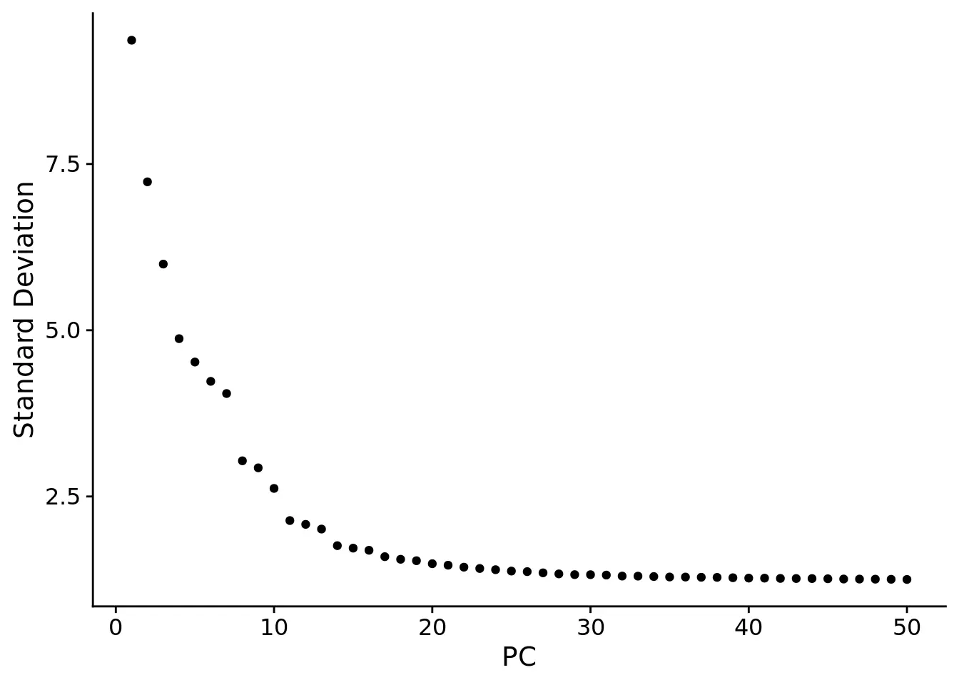
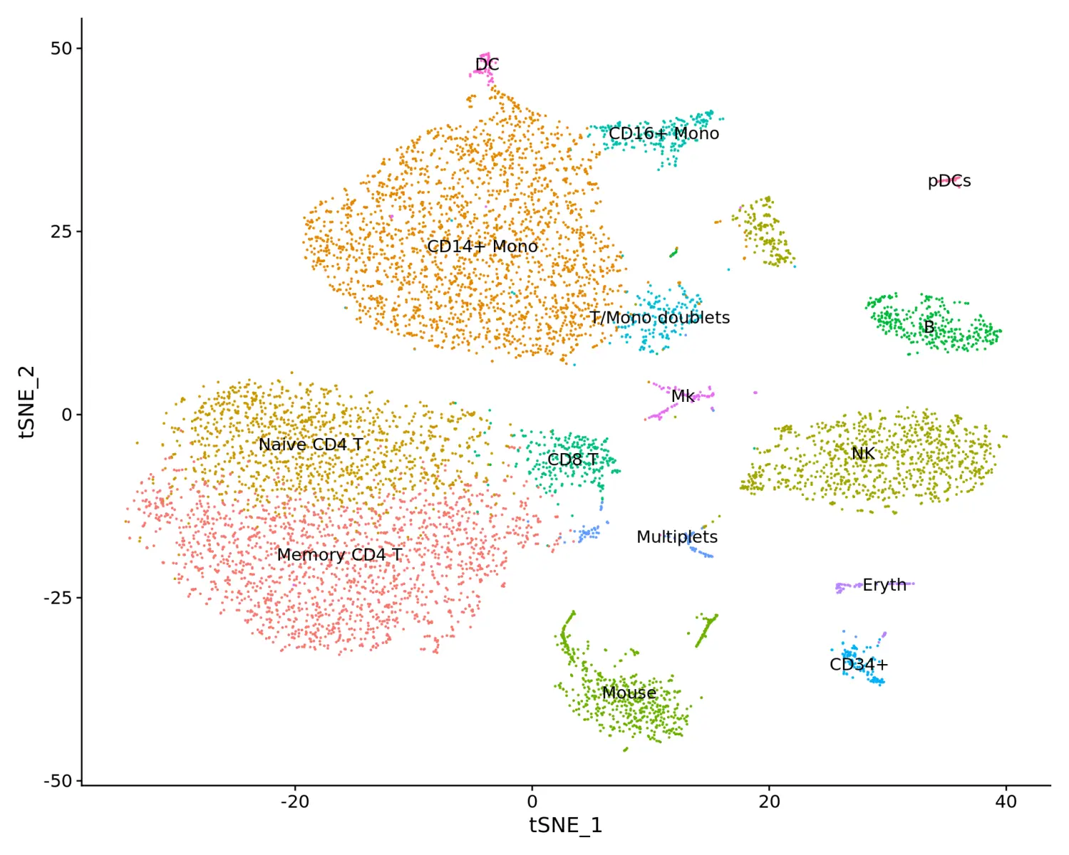
# 使用图聚类进行细胞分群cbmc <- FindNeighbors(cbmc, dims = 1:25)cbmc <- FindClusters(cbmc, resolution = 0.8)# tSNE降维可视化cbmc <- RunTSNE(cbmc, dims = 1:25, method = "FIt-SNE")# Find the markers that define each cluster, and use these to annotate the clusters, we use max.cells.per.ident to speed up the process# 鉴定差异表达基因cbmc.rna.markers <- FindAllMarkers(cbmc, max.cells.per.ident = 100, min.diff.pct = 0.3, only.pos = TRUE)# Note, for simplicity we are merging two CD14+ Monocyte clusters (that differ in expression of HLA-DR genes) and NK clusters (that differ in cell cycle stage)# 细胞分群重命名new.cluster.ids <- c("Memory CD4 T", "CD14+ Mono", "Naive CD4 T", "NK", "CD14+ Mono", "Mouse", "B", "CD8 T", "CD16+ Mono", "T/Mono doublets", "NK", "CD34+", "Multiplets", "Mouse", "Eryth", "Mk", "Mouse", "DC", "pDCs")names(new.cluster.ids) <- levels(cbmc)cbmc <- RenameIdents(cbmc, new.cluster.ids)# 数据可视化DimPlot(cbmc, label = TRUE) + NoLegend()
将蛋白的表达水平添加到Seurat对象中
Seurat3可以将多个不同assay的信息存储到同一个对象中,只要数据是多模式的(在同一组细胞上收集)即可。我们可以使用SetAssayData和GetAssayData函数将其他assay的信息添加到seurat对象中。
# We will define an ADT assay, and store raw counts for it# If you are interested in how these data are internally stored, you can check out the Assay class, which is defined in objects.R; note that all single-cell expression data, including RNA data, are still stored in Assay objects, and can also be accessed using GetAssayData# 构建新的Assay对象cbmc[["ADT"]] <- CreateAssayObject(counts = cbmc.adt)# Now we can repeat the preprocessing (normalization and scaling) steps that we typically run with RNA, but modifying the 'assay' argument. For CITE-seq data, we do not recommend typical LogNormalization. Instead, we use a centered log-ratio (CLR) normalization, computed independently for each feature. This is a slightly improved procedure from the original publication, and we will release more advanced versions of CITE-seq normalizations soon.# 使用“CLR”方法进行数据归一化cbmc <- NormalizeData(cbmc, assay = "ADT", normalization.method = "CLR")cbmc <- ScaleData(cbmc, assay = "ADT")
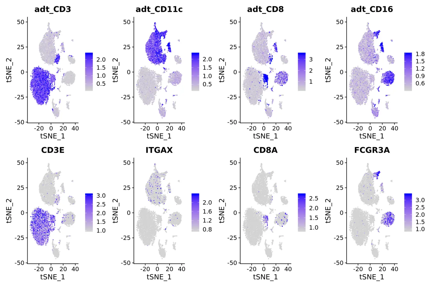
在RNA表达分群的基础上可视化蛋白的定量水平
# in this plot, protein (ADT) levels are on top, and RNA levels are on the bottom# 其中带有adt_前缀的基因即为蛋白的表达水平FeaturePlot(cbmc, features = c("adt_CD3", "adt_CD11c", "adt_CD8", "adt_CD16", "CD3E", "ITGAX", "CD8A", "FCGR3A"), min.cutoff = "q05", max.cutoff = "q95", ncol = 4)
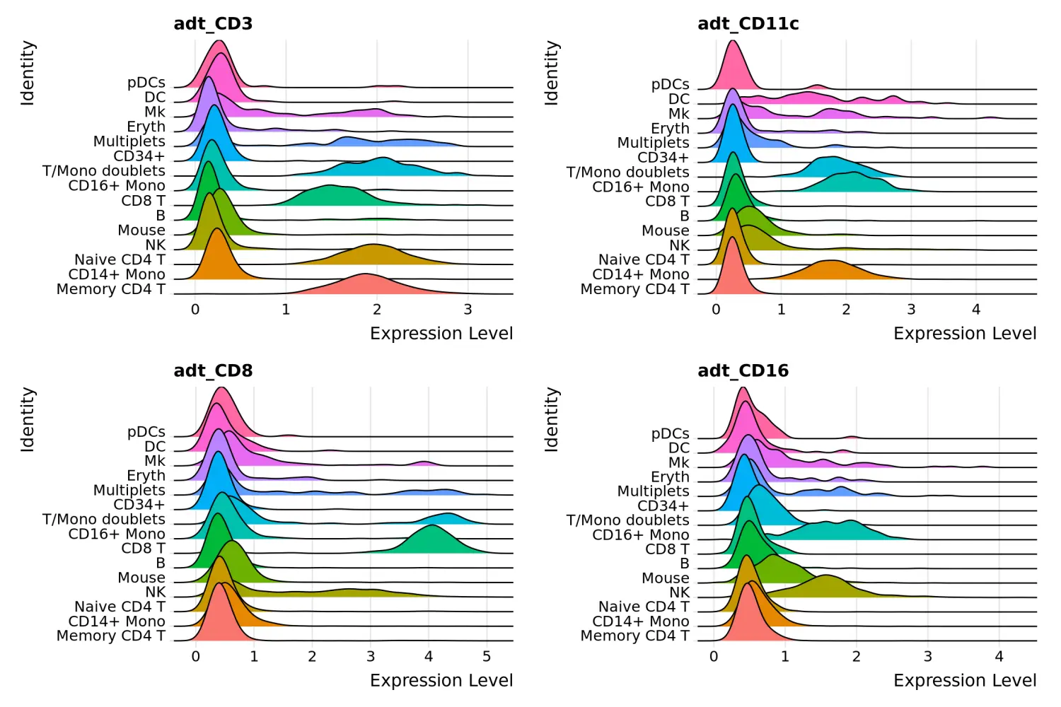
RidgePlot(cbmc, features = c("adt_CD3", "adt_CD11c", "adt_CD8", "adt_CD16"), ncol = 2)
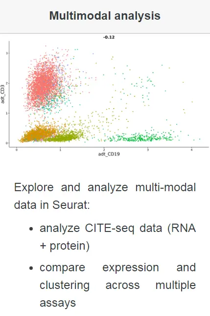
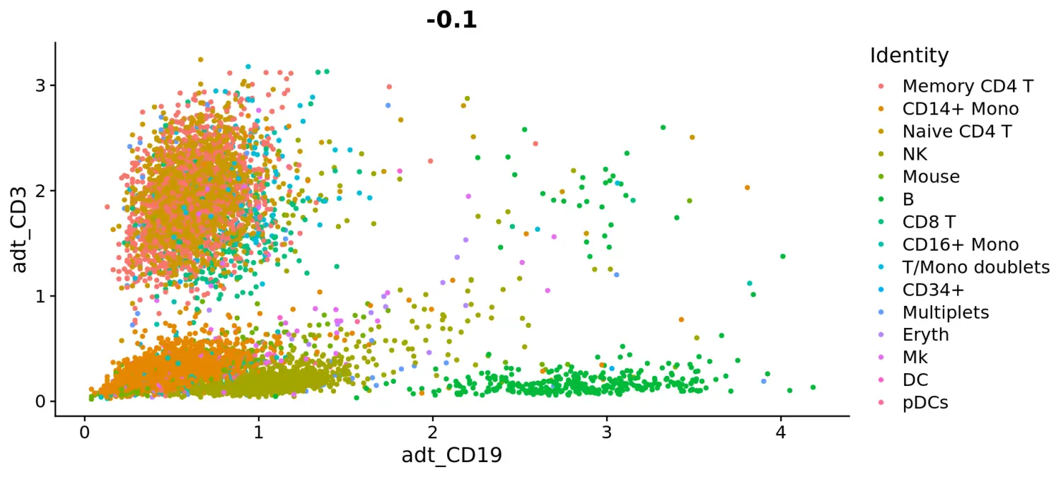
# Draw ADT scatter plots (like biaxial plots for FACS). Note that you can even 'gate' cells if desired by using HoverLocator and FeatureLocatorFeatureScatter(cbmc, feature1 = "adt_CD19", feature2 = "adt_CD3")
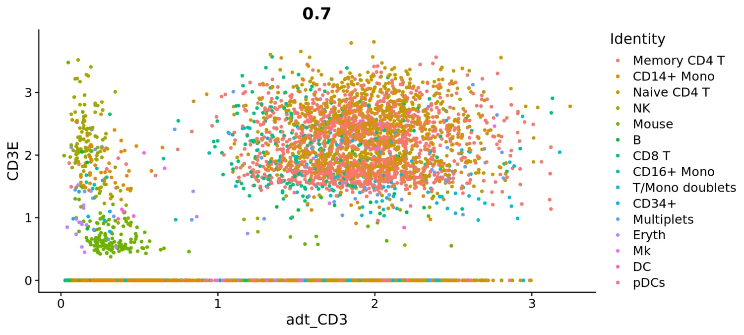
# view relationship between protein and RNAFeatureScatter(cbmc, feature1 = "adt_CD3", feature2 = "CD3E")
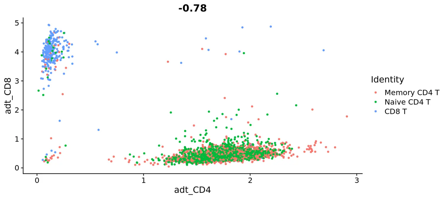
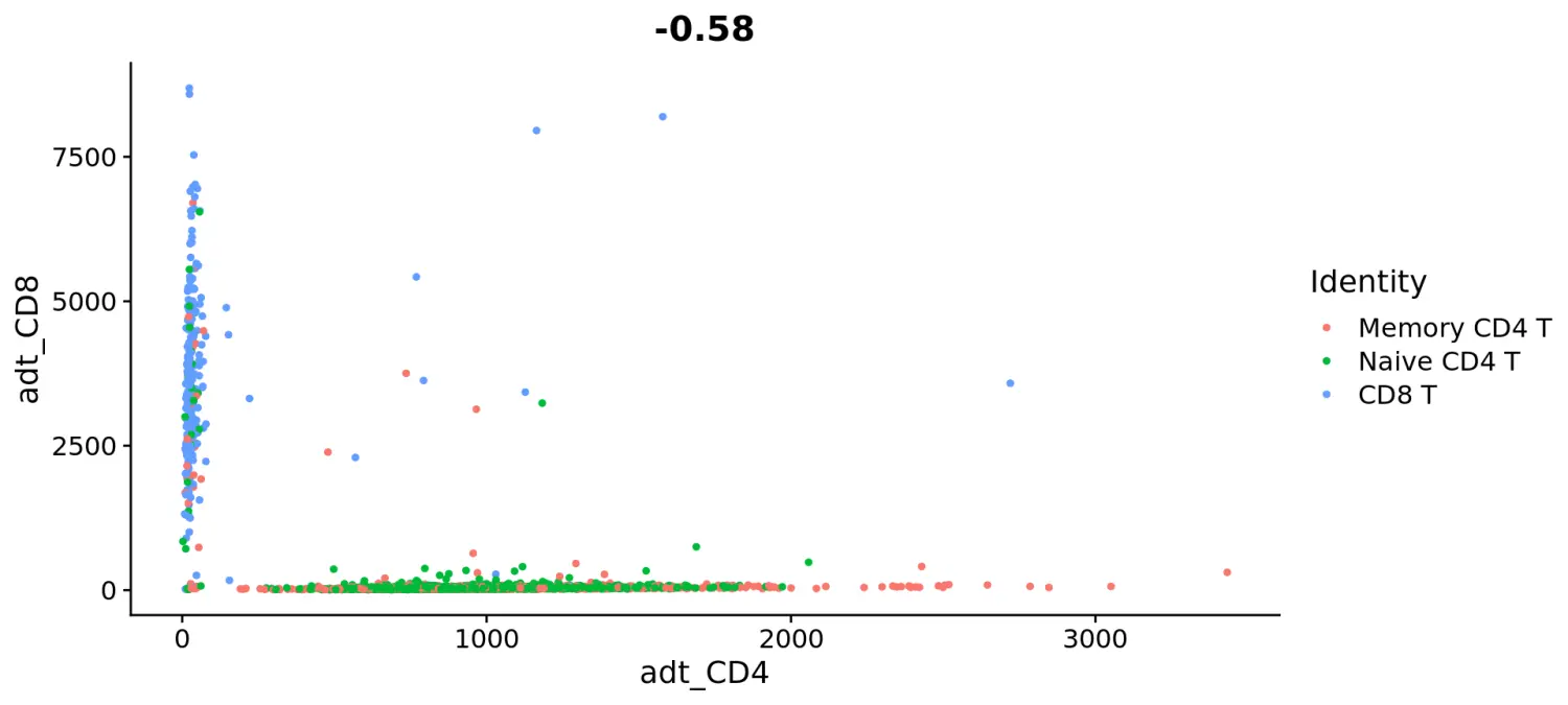
# Let's plot CD4 vs CD8 levels in T cellstcells <- subset(cbmc, idents = c("Naive CD4 T", "Memory CD4 T", "CD8 T"))FeatureScatter(tcells, feature1 = "adt_CD4", feature2 = "adt_CD8")
# Let's look at the raw (non-normalized) ADT counts. You can see the values are quite high, particularly in comparison to RNA values. This is due to the significantly higher protein copy number in cells, which significantly reduces 'drop-out' in ADT dataFeatureScatter(tcells, feature1 = "adt_CD4", feature2 = "adt_CD8", slot = "counts")saveRDS(cbmc, file = "../output/cbmc.rds")
鉴定不同细胞分群之间差异表达的蛋白
# Downsample the clusters to a maximum of 300 cells each (makes the heatmap easier to see for small clusters)
cbmc.small <- subset(cbmc, downsample = 300)

# Find protein markers for all clusters, and draw a heatmap
adt.markers <- FindAllMarkers(cbmc.small, assay = "ADT", only.pos = TRUE)
DoHeatmap(cbmc.small, features = unique(adt.markers$gene), assay = "ADT", angle = 90) + NoLegend()
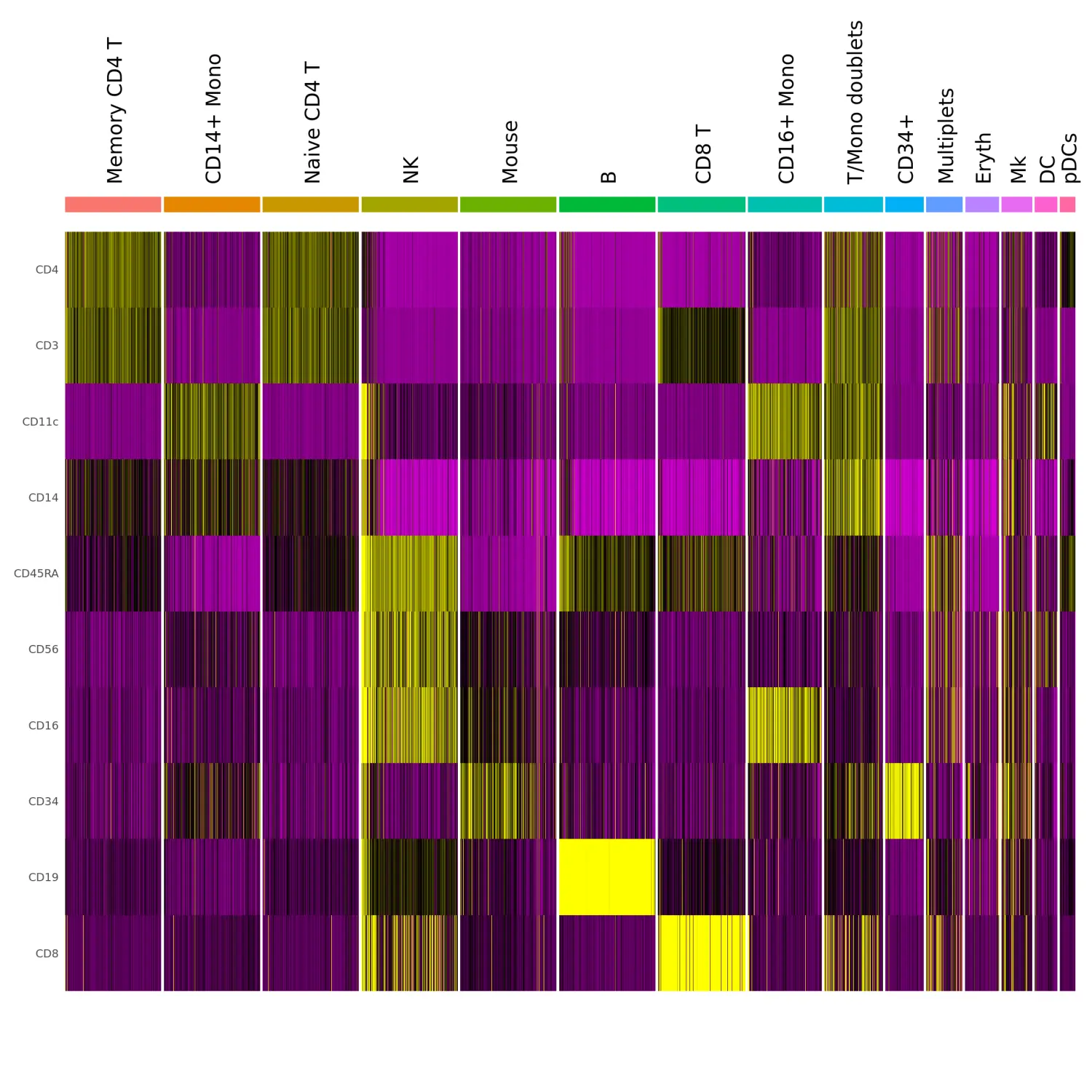
# You can see that our unknown cells co-express both myeloid and lymphoid markers (true at the RNA level as well). They are likely cell clumps (multiplets) that should be discarded. We'll remove the mouse cells now as well
cbmc <- subset(cbmc, idents = c("Multiplets", "Mouse"), invert = TRUE)
根据蛋白的表达水平进行聚类分群
# Because we're going to be working with the ADT data extensively, we're going to switch the default assay to the 'CITE' assay.  This will cause all functions to use ADT data by default, rather than requiring us to specify it each time
# 将默认的Assay更换为"ADT"的数据
DefaultAssay(cbmc) <- "ADT"
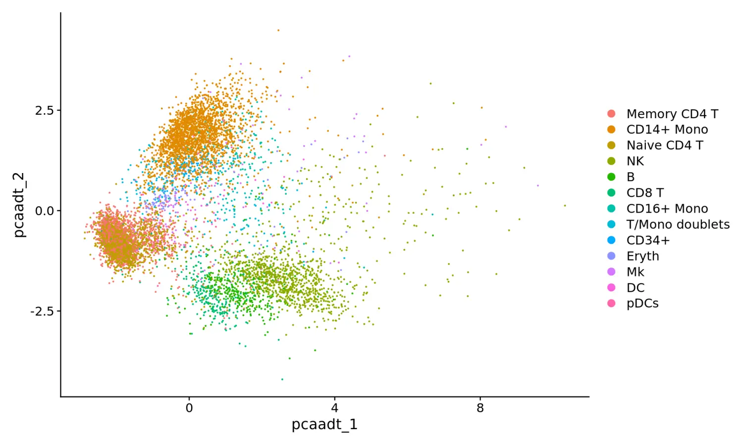
# PCA降维
cbmc <- RunPCA(cbmc, features = rownames(cbmc), reduction.name = "pca_adt", reduction.key = "pca_adt_", verbose = FALSE)
# PCA降维可视化
DimPlot(cbmc, reduction = "pca_adt")
# Since we only have 10 markers, instead of doing PCA, we'll just use a standard euclidean distance matrix here.  Also, this provides a good opportunity to demonstrate how to do visualization and clustering using a custom distance matrix in Seurat
adt.data <- GetAssayData(cbmc, slot = "data")
adt.dist <- dist(t(adt.data))

# Before we recluster the data on ADT levels, we'll stash the RNA cluster IDs for later
cbmc[["rnaClusterID"]] <- Idents(cbmc)

# Now, we rerun tSNE using our distance matrix defined only on ADT (protein) levels.
cbmc[["tsne_adt"]] <- RunTSNE(adt.dist, assay = "ADT", reduction.key = "adtTSNE_")
cbmc[["adt_snn"]] <- FindNeighbors(adt.dist)$snn
cbmc <- FindClusters(cbmc, resolution = 0.2, graph.name = "adt_snn")

# We can compare the RNA and protein clustering, and use this to annotate the protein clustering (we could also of course use FindMarkers)
clustering.table <- table(Idents(cbmc), cbmc$rnaClusterID)
clustering.table
new.cluster.ids <- c("CD4 T", "CD14+ Mono", "NK", "B", "CD8 T", "NK", "CD34+", "T/Mono doublets", "CD16+ Mono", "pDCs", "B")
names(new.cluster.ids) <- levels(cbmc)
cbmc <- RenameIdents(cbmc, new.cluster.ids)

tsne_rnaClusters <- DimPlot(cbmc, reduction = "tsne_adt", group.by = "rnaClusterID") + NoLegend()
tsne_rnaClusters <- tsne_rnaClusters + ggtitle("Clustering based on scRNA-seq") + theme(plot.title = element_text(hjust = 0.5))
tsne_rnaClusters <- LabelClusters(plot = tsne_rnaClusters, id = "rnaClusterID", size = 4)

tsne_adtClusters <- DimPlot(cbmc, reduction = "tsne_adt", pt.size = 0.5) + NoLegend()
tsne_adtClusters <- tsne_adtClusters + ggtitle("Clustering based on ADT signal") + theme(plot.title = element_text(hjust = 0.5))
tsne_adtClusters <- LabelClusters(plot = tsne_adtClusters, id = "ident", size = 4)

# Note: for this comparison, both the RNA and protein clustering are visualized on a tSNE generated using the ADT distance matrix.
wrap_plots(list(tsne_rnaClusters, tsne_adtClusters), ncol = 2)
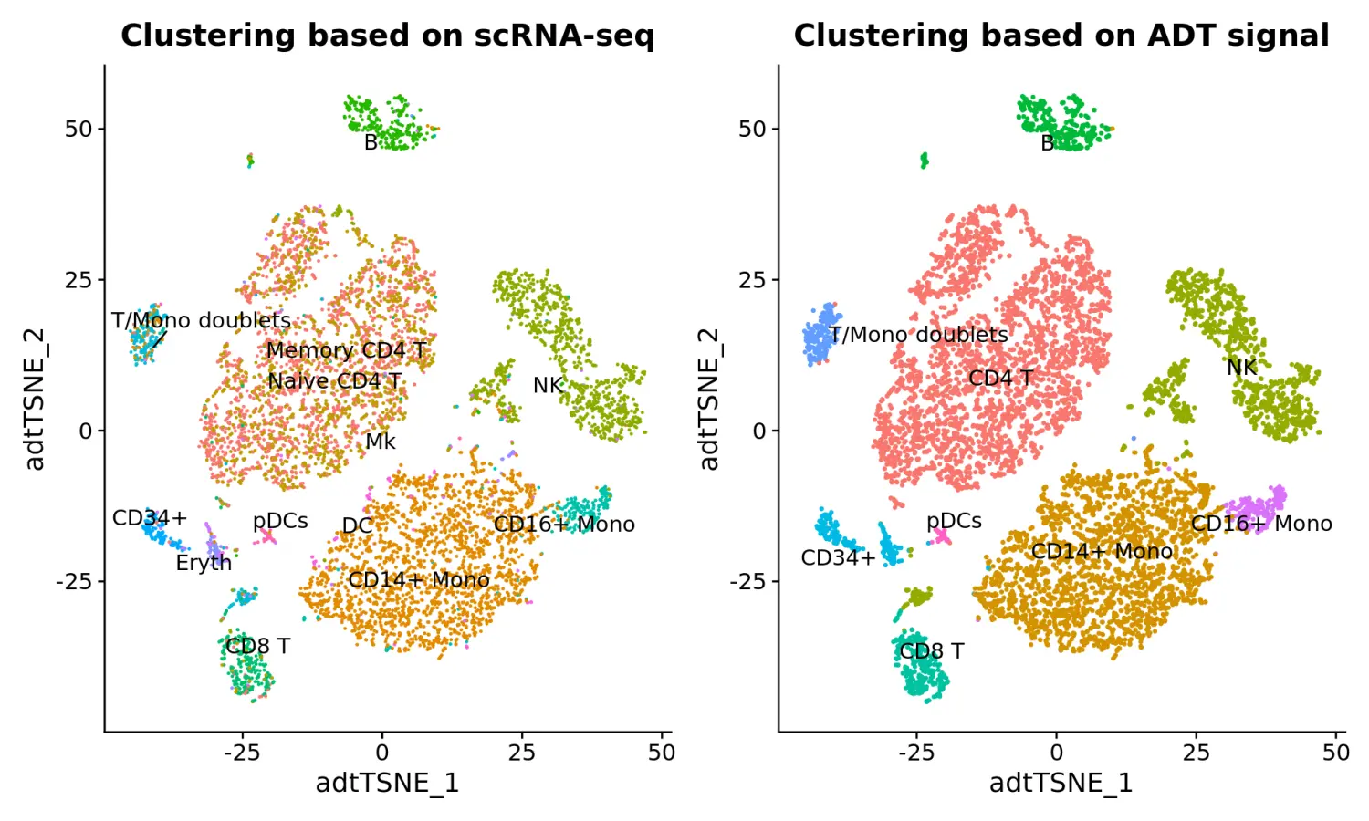
从上图可以看出,基于ADT的蛋白水平聚类结果和基因表达的scRNA-seq产生相似的结果,但仍有一些区别:
- Clustering is improved for CD4/CD8 T cell populations, based on the robust ADT data for CD4, CD8, CD14, and CD45RA
- However, some clusters for which the ADT data does not contain good distinguishing protein markers (i.e. Mk/Ery/DC) lose separation
- You can verify this using FindMarkers at the RNA level, as well
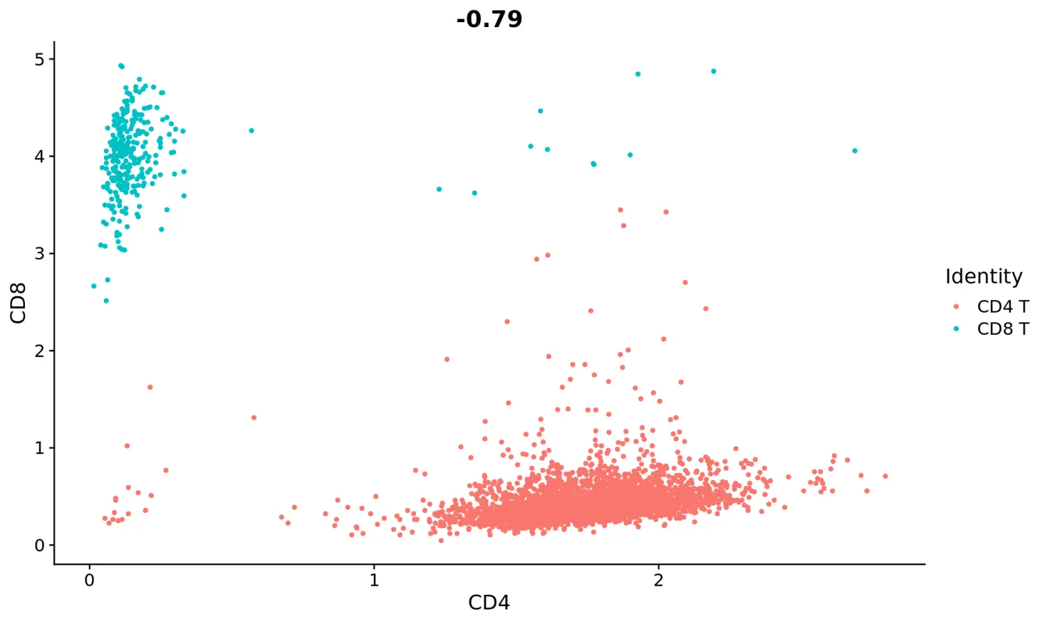
tcells <- subset(cbmc, idents = c("CD4 T", "CD8 T"))
FeatureScatter(tcells, feature1 = "CD4", feature2 = "CD8")
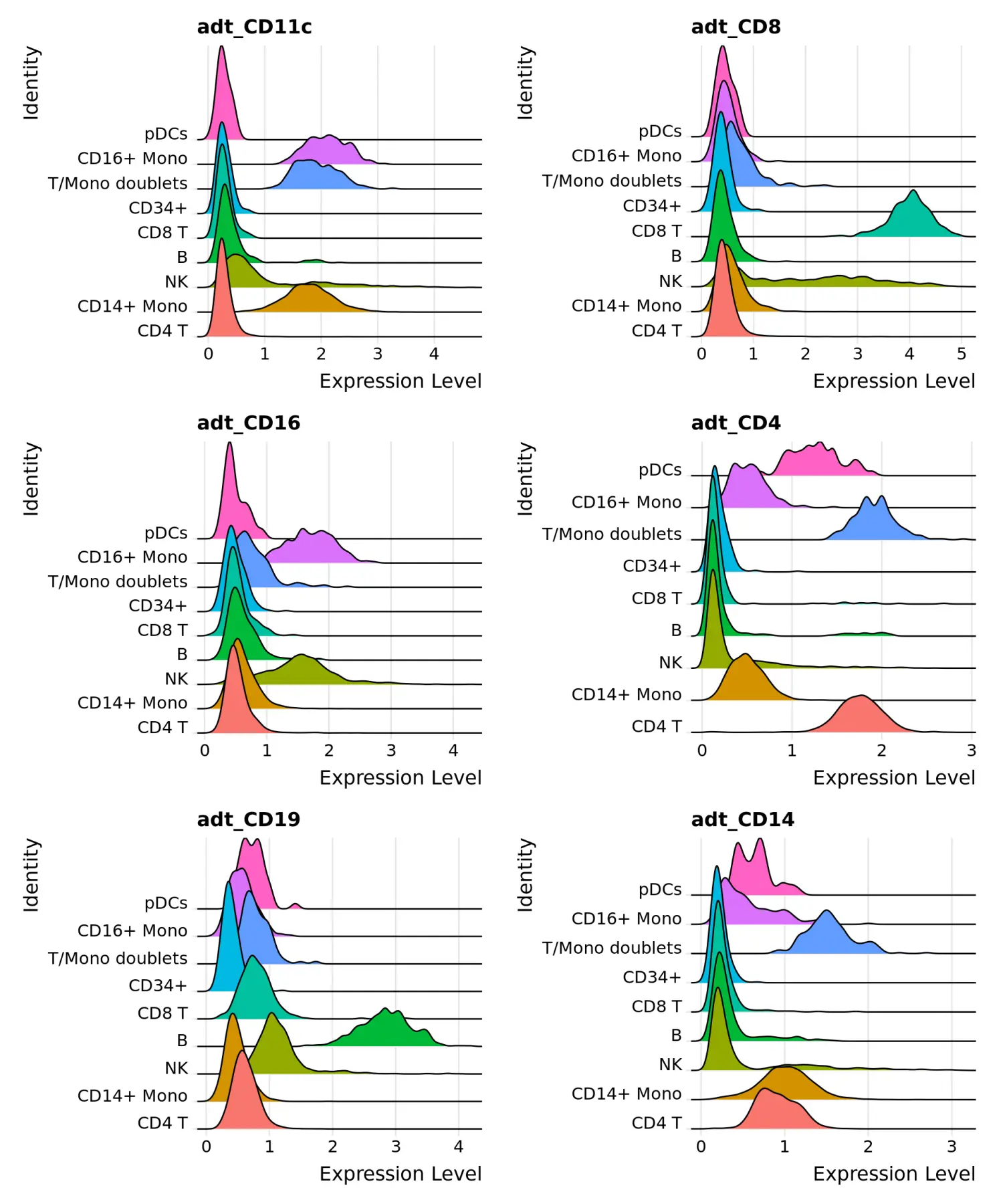
RidgePlot(cbmc, features = c("adt_CD11c", "adt_CD8", "adt_CD16", "adt_CD4", "adt_CD19", "adt_CD14"), ncol = 2)
# 保存分析好的数据
saveRDS(cbmc, file = "../output/cbmc_multimodal.rds")
加载10x genomics多模式实验产生的数据
Seurat3还能够分析使用CellRanger v3处理的多模式10X实验产生的数据;例如,我们使用7,900个外周血单核细胞(PBMC)的数据集(10X Genomics平台产生)重新完成上述的分析流程。
# 读取cellranger处理生成的表达矩阵
pbmc10k.data <- Read10X(data.dir = "../data/pbmc10k/filtered_feature_bc_matrix/")

rownames(x = pbmc10k.data[["Antibody Capture"]]) <- gsub(pattern = "_[control_]*TotalSeqB", replacement = "", x = rownames(x = pbmc10k.data[["Antibody Capture"]]))
# 构建seurat对象
pbmc10k <- CreateSeuratObject(counts = pbmc10k.data[["Gene Expression"]], min.cells = 3, min.features = 200)
# 数据标准化
pbmc10k <- NormalizeData(pbmc10k)
# 新建蛋白定量的ADT对象
pbmc10k[["ADT"]] <- CreateAssayObject(pbmc10k.data[["Antibody Capture"]][, colnames(x = pbmc10k)])
# 数据标准化
pbmc10k <- NormalizeData(pbmc10k, assay = "ADT", normalization.method = "CLR")

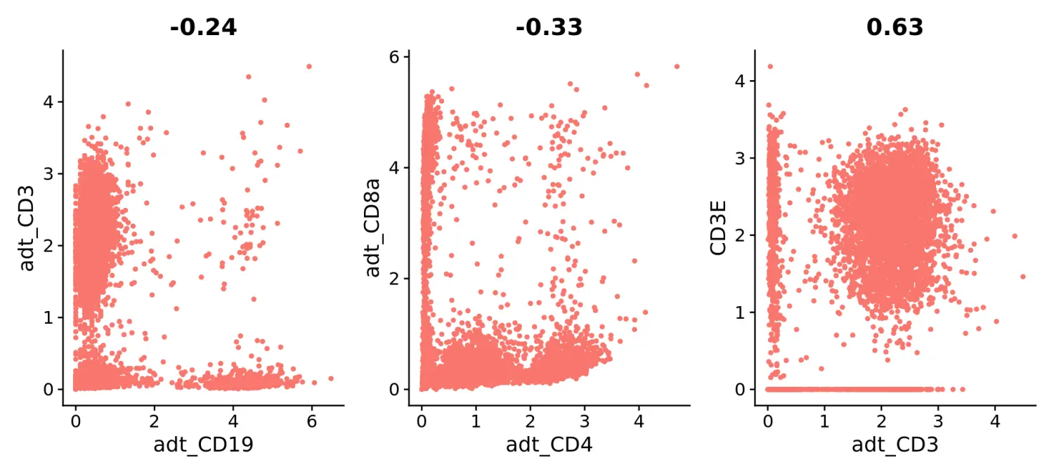
plot1 <- FeatureScatter(pbmc10k, feature1 = "adt_CD19", feature2 = "adt_CD3", pt.size = 1)
plot2 <- FeatureScatter(pbmc10k, feature1 = "adt_CD4", feature2 = "adt_CD8a", pt.size = 1)
plot3 <- FeatureScatter(pbmc10k, feature1 = "adt_CD3", feature2 = "CD3E", pt.size = 1)
(plot1 + plot2 + plot3) & NoLegend()
参考来源:https://satijalab.org/seurat/v3.1/multimodal_vignette.html

