自实现PCA

PCA模型封装

import numpy as np
class PCA:
    def __init__(self, n_components):
        """初始化PCA"""
        assert n_components >= 1, "n_components must be valid"
        self.n_components = n_components
        self.components_ = None
    def fit(self, X, eta=0.01, n_iters=1e4):
        """获得数据集X的前n个主成分"""
        assert self.n_components <= X.shape[1], \
            "n_components must not be greater than the feature number of X"
        def demean(X):
            return X - np.mean(X, axis=0)
        def f(w, X):
            return np.sum((X.dot(w) ** 2)) / len(X)
        def df(w, X):
            return X.T.dot(X.dot(w)) * 2. / len(X)
        def direction(w):
            return w / np.linalg.norm(w)
        def first_component(X, initial_w, eta=0.01, n_iters=1e4, epsilon=1e-8):
            w = direction(initial_w)
            cur_iter = 0
            while cur_iter < n_iters:
                gradient = df(w, X)
                last_w = w
                w = w + eta * gradient
                w = direction(w)
                if (abs(f(w, X) - f(last_w, X)) < epsilon):
                    break
                cur_iter += 1
            return w
        X_pca = demean(X)
        self.components_ = np.empty(shape=(self.n_components, X.shape[1]))
        for i in range(self.n_components):
            initial_w = np.random.random(X_pca.shape[1])
            w = first_component(X_pca, initial_w, eta, n_iters)
            self.components_[i,:] = w
            X_pca = X_pca - X_pca.dot(w).reshape(-1, 1) * w
        return self
    def transform(self, X):
        """将给定的X，映射到各个主成分分量中"""
        assert X.shape[1] == self.components_.shape[1]
        return X.dot(self.components_.T)
    def inverse_transform(self, X):
        """将给定的X，反向映射回原来的特征空间"""
        assert X.shape[1] == self.components_.shape[0]
        return X.dot(self.components_)
    def __repr__(self):
        return "PCA(n_components=%d)" % self.n_components

使用

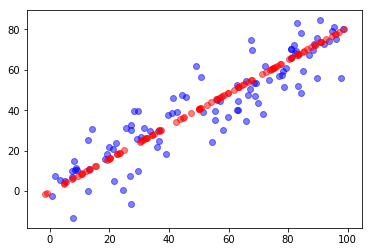
import numpy as np
import matplotlib.pyplot as plt
# 准备数据
X = np.empty((100, 2))
X[:,0] = np.random.uniform(0., 100., size=100)
X[:,1] = 0.75 * X[:,0] + 3. + np.random.normal(0, 10., size=100)
# 求解2个主成分
from playML.PCA import PCA
pca = PCA(n_components=2)
pca.fit(X)
pca.components_  # array([[ 0.76676948,  0.64192256], [-0.64191827,  0.76677307]])
#  求解第一主成分
pca = PCA(n_components=1)
pca.fit(X)
# 将数据降维(高维转为低维)
X_reduction = pca.transform(X)  # X_reduction.shape ： (100, 1)
# 将数据还原(低维转为高维)
X_restore = pca.inverse_transform(X_reduction)  # X_restore.shape ： (100, 2)
# 可视化
# # 蓝色代表原数据，红色代表降维后在第一维的数据
plt.scatter(X[:,0], X[:,1], color='b', alpha=0.5)
plt.scatter(X_restore[:,0], X_restore[:,1], color='r', alpha=0.5)
plt.show()

scikit-learn实现PCA

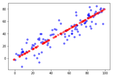
from sklearn.decomposition import PCA
# 降维
pca = PCA(n_components=1)
pca.fit(X)
# 求解第一主成分
pca.components_  # array([[-0.77670058, -0.62987   ]])
# 将数据降维(高维转为低维)
X_reduction = pca.transform(X)
# 将数据还原(低维转为高维)
X_restore = pca.inverse_transform(X_reduction)
# 可视化
# # 蓝色代表原数据，红色代表降维后在第一维的数据
plt.scatter(X[:,0], X[:,1], color='b', alpha=0.5)
plt.scatter(X_restore[:,0], X_restore[:,1], color='r', alpha=0.5)
plt.show()