-
梯度上升法和梯度下降法一样的,差别就是反向了,减法改为了加法。 - 效用函数也叫目标函数。
准备数据
```python import numpy as np import matplotlib.pyplot as plt
准备数据
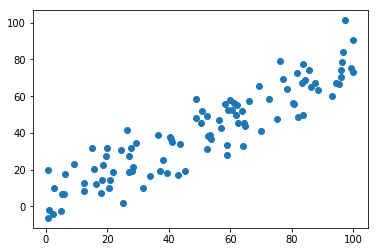
X = np.empty((100, 2)) X[:,0] = np.random.uniform(0., 100., size=100) # 第一列 X[:,1] = 0.75 * X[:,0] + 3. + np.random.normal(0, 10., size=100) # 第二列
plt.scatter(X[:,0], X[:,1]) plt.show()
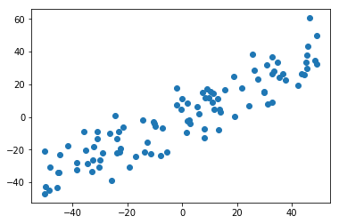
<a name="RgYlw"></a># 数据预处理<a name="IL1xD"></a>## demean均值归零:把样本点移动到坐标系原点附近。```pythondef demean(X):return X - np.mean(X, axis=0)X_demean = demean(X)plt.scatter(X_demean[:,0], X_demean[:,1])plt.show()
# 检查预处理结果:两列均值均接近0np.mean(X_demean[:,0]) # 8.171241461241152e-15np.mean(X_demean[:,1]) # -1.0231815394945442e-14
模型封装
def f(w, X):'''目标函数'''return np.sum((X.dot(w)**2)) / len(X)def df_math(w, X):'''目标函数的梯度: 矩阵实现'''return X.T.dot(X.dot(w)) * 2. / len(X)def df_debug(w, X, epsilon=0.0001):'''目标函数的梯度:迭代实现'''res = np.empty(len(w))for i in range(len(w)):w_1 = w.copy()w_1[i] += epsilonw_2 = w.copy()w_2[i] -= epsilonres[i] = (f(w_1, X) - f(w_2, X)) / (2 * epsilon)return resdef direction(w):'''w的单位向量'''return w / np.linalg.norm(w)def gradient_ascent(df, X, initial_w, eta, n_iters = 1e4, epsilon=1e-8):'''目标函数的梯度上升法'''w = direction(initial_w)cur_iter = 0while cur_iter < n_iters:gradient = df(w, X)last_w = ww = w + eta * gradientw = direction(w) # 注意1:每次求一个单位方向if(abs(f(w, X) - f(last_w, X)) < epsilon):breakcur_iter += 1return w
编码实现
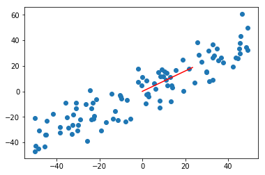
# 建模initial_w = np.random.random(X.shape[1]) # 注意2:不能用0向量开始initial_w # array([0.19082376, 0.43894239])eta = 0.001## 注意3: 不能使用StandardScaler标准化数据w = gradient_ascent(df_debug, X_demean, initial_w, eta) # array([0.78159851, 0.62378183])w = gradient_ascent(df_debug, X_demean, initial_w, eta) # array([0.78159851, 0.62378183])# 可视化plt.scatter(X_demean[:,0], X_demean[:,1])plt.plot([0, w[0]*30], [0, w[1]*30], color='r')plt.show()
极端数据集测试
准备数据
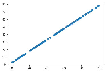
X2 = np.empty((100, 2))X2[:,0] = np.random.uniform(0., 100., size=100)X2[:,1] = 0.75 * X2[:,0] + 3.plt.scatter(X2[:,0], X2[:,1])plt.show()
预处理
X2_demean = demean(X2)np.mean(X_demean[:,0]) # 8.171241461241152e-15np.mean(X_demean[:,1]) # -1.0231815394945442e-14
建模
w2 = gradient_ascent(df_math, X2_demean, initial_w, eta)
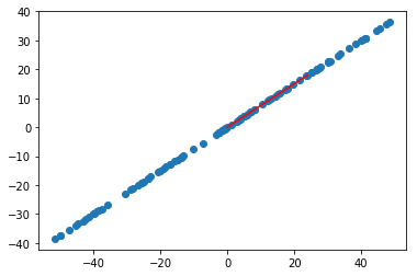
可视化
plt.scatter(X2_demean[:,0], X2_demean[:,1]) # 样本点plt.plot([0, w2[0]*30], [0, w2[1]*30], color='r') # PCA向量plt.show()
和梯度下降法一样,梯度上升法 也有随机梯度和小批量梯度。

若有收获,就点个赞吧
0 人点赞
