定义:将样本的特征和样本发生的概率联系起来,概率是一个数
作用:通常用做分类算法,只能解决二分类问题
1.原理
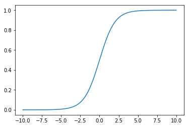
1.1 sigmoid 函数
-
 ```python
import numpy as np
import matplotlib.pyplot as plt
```python
import numpy as np
import matplotlib.pyplot as plt
def sigmoid(t): return 1. / (1. + np.exp(-t))
x = np.linspace(-10, 10, 500)
plt.plot(x, sigmoid(x)) plt.show()
<a name="jA53u"></a>## 1.2 sigmoid 结合线性回归- [x] 令 ,- [x] 再将概率对应取值:<a name="pQi7k"></a>## 1.3 损失函数<br />如何用公式表示这样的损失函数?<a name="vKvOX"></a>### 单个值的损失函数<br />分段函数不好用,能不能结合成一个函数表示?<br /><br />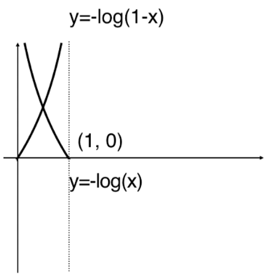<a name="gTE7A"></a>### 损失函数的平均值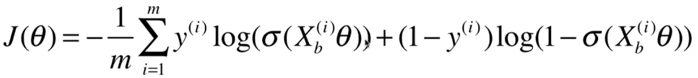<br />损失函数没有公式解,只能用梯度下降法求解。<a name="DBJ5i"></a>## 1.4 损失函数的梯度<a name="F4giF"></a># 2.编码<a name="impSD"></a>## 2.1 自定义模型封装```pythonimport numpy as npfrom .metrics import accuracy_scoreclass LogisticRegression:def __init__(self):"""初始化Logistic Regression模型"""self.coef_ = Noneself.intercept_ = Noneself._theta = Nonedef _sigmoid(self, t):return 1. / (1. + np.exp(-t))def fit(self, X_train, y_train, eta=0.01, n_iters=1e4):"""根据训练数据集X_train, y_train, 使用梯度下降法训练Logistic Regression模型"""assert X_train.shape[0] == y_train.shape[0], \"the size of X_train must be equal to the size of y_train"def J(theta, X_b, y):y_hat = self._sigmoid(X_b.dot(theta))try:return - np.sum(y*np.log(y_hat) + (1-y)*np.log(1-y_hat)) / len(y)except:return float('inf')def dJ(theta, X_b, y):return X_b.T.dot(self._sigmoid(X_b.dot(theta)) - y) / len(y)def gradient_descent(X_b, y, initial_theta, eta, n_iters=1e4, epsilon=1e-8):theta = initial_thetacur_iter = 0while cur_iter < n_iters:gradient = dJ(theta, X_b, y)last_theta = thetatheta = theta - eta * gradientif (abs(J(theta, X_b, y) - J(last_theta, X_b, y)) < epsilon):breakcur_iter += 1return thetaX_b = np.hstack([np.ones((len(X_train), 1)), X_train])initial_theta = np.zeros(X_b.shape[1])self._theta = gradient_descent(X_b, y_train, initial_theta, eta, n_iters)self.intercept_ = self._theta[0]self.coef_ = self._theta[1:]return selfdef predict_proba(self, X_predict):"""给定待预测数据集X_predict,返回表示X_predict的结果概率向量"""assert self.intercept_ is not None and self.coef_ is not None, \"must fit before predict!"assert X_predict.shape[1] == len(self.coef_), \"the feature number of X_predict must be equal to X_train"X_b = np.hstack([np.ones((len(X_predict), 1)), X_predict])return self._sigmoid(X_b.dot(self._theta))def predict(self, X_predict):"""给定待预测数据集X_predict,返回表示X_predict的结果向量"""assert self.intercept_ is not None and self.coef_ is not None, \"must fit before predict!"assert X_predict.shape[1] == len(self.coef_), \"the feature number of X_predict must be equal to X_train"proba = self.predict_proba(X_predict)return np.array(proba >= 0.5, dtype='int')def score(self, X_test, y_test):"""根据测试数据集 X_test 和 y_test 确定当前模型的准确度"""y_predict = self.predict(X_test)return accuracy_score(y_test, y_predict)def __repr__(self):return "LogisticRegression()"
2.2 建模
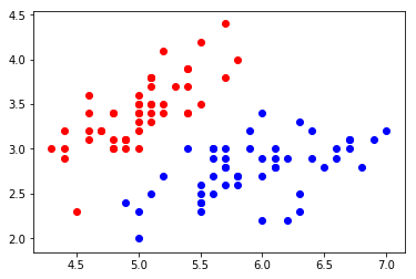
# 1.数据准备import numpy as npimport matplotlib.pyplot as pltfrom sklearn import datasetsiris = datasets.load_iris()X = iris.datay = iris.target# 选择两个分类X = X[y<2,:2]y = y[y<2]# 2.可视化plt.scatter(X[y==0,0], X[y==0,1], color="red")plt.scatter(X[y==1,0], X[y==1,1], color="blue")plt.show()
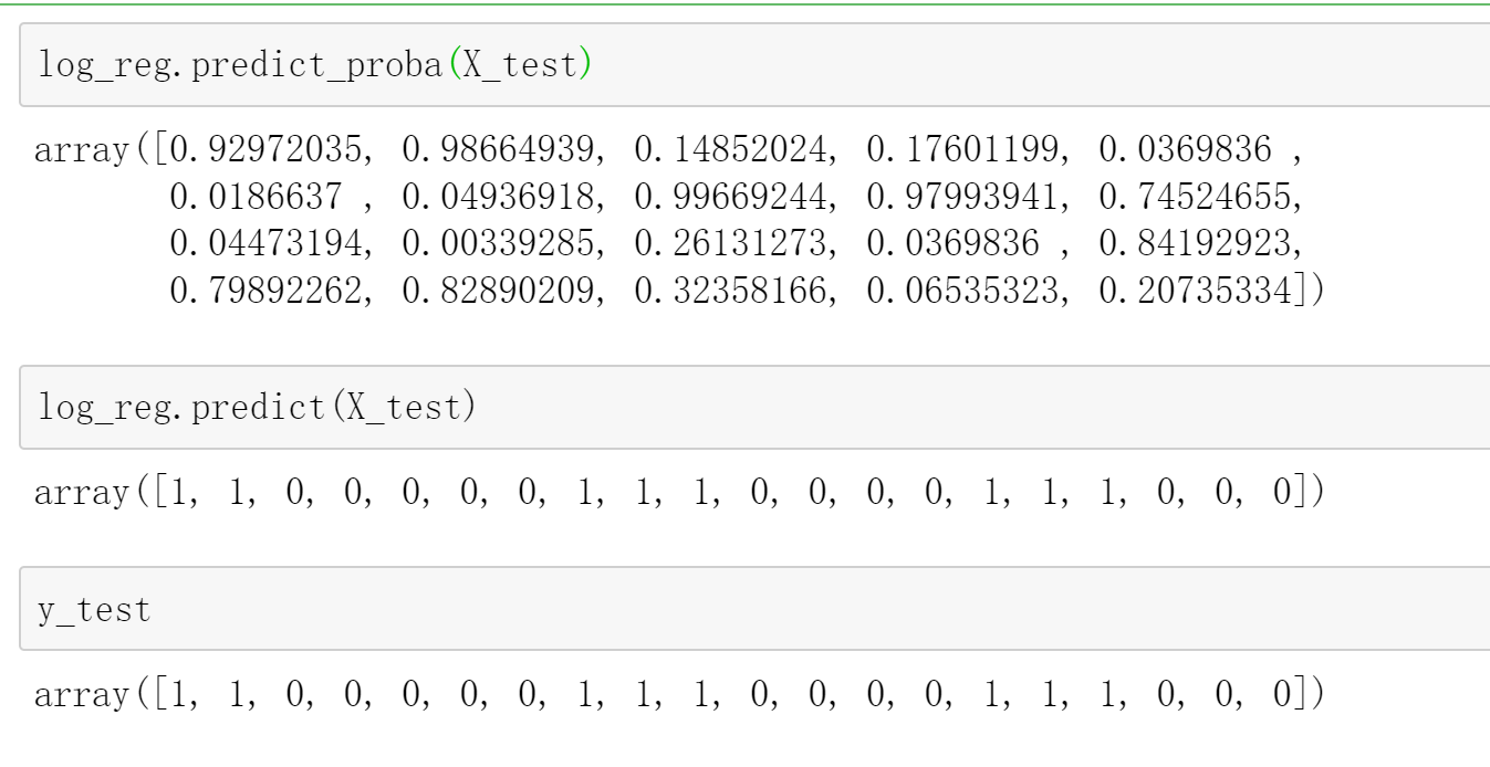
# 3.数据分割from playML.model_selection import train_test_splitX_train, X_test, y_train, y_test = train_test_split(X, y, seed=666)# 4.建模from playML.LogisticRegression import LogisticRegressionlog_reg = LogisticRegression()log_reg.fit(X_train, y_train)log_reg.score(X_test, y_test) # 模型准确度: 1.0#5. 预测

若有收获,就点个赞吧
0 人点赞
