R-FCN: 20 May 2016

R-FCN: Object Detection via Region-based Fully Convolutional Networks

Abstract

In contrast to previous region-based detectors such as Fast/Faster R-CNN [6, 18] that apply a costly per-region subnetwork hundreds of times, our region-based detector is fully convolutional with almost all computation shared on the entire image. To achieve this goal, we propose position-sensitive score maps to address a dilemma（困境） between translation-invariance in image classification and translation-variance in object detection. Meanwhile, our result is achieved at a test-time speed of 170ms per image, 2.5-20× faster than the Faster R-CNN counterpart.

1. Introduction

A prevalent family [8, 6, 18] of deep networks for object detection can be divided into two subnetworks by the Region-of-Interest (RoI) pooling layer [6]: (i) a shared, “fully convolutional” subnetwork independent of RoIs, and (ii) an RoI-wise subnetwork that does not share computation.
In this paper, we develop a framework called Region-based Fully Convolutional Network (R-FCN) for object detection. Our network consists of shared, fully convolutional architectures as is the case of FCN [15]. To incorporate translation variance（平移可变性） into FCN, we construct a set of position-sensitive score maps by using a bank of specialized convolutional layers as the FCN output. Each of these score maps encodes the position information with respect to a relative spatial position (e.g., “to the left of an object”). On top of this FCN, we append a position-sensitive RoI pooling layer that shepherds information from these score maps, with no weight (convolutional/fc) layers following. The entire architecture is learned end-to-end. All learnable layers are convolutional and shared on the entire image, yet encode spatial information required for object detection. Figure 1 illustrates the key idea and Table 1 compares the methodologies among region-based detectors.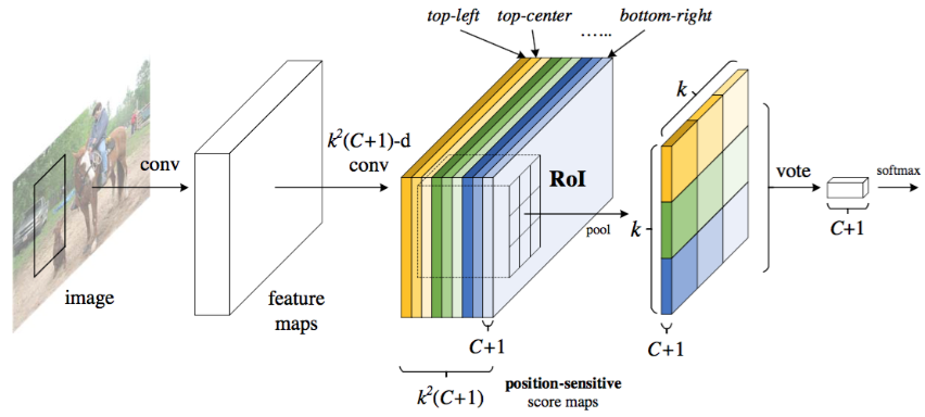

Figure 1: Key idea of R-FCN for object detection. In this illustration, there are k × k = 3 × 3 position-sensitive score maps generated by a fully convolutional network. For each of the k × k bins in an RoI, pooling is only performed on one of the k^2 maps (marked by different colors).
Following R-CNN [7], we adopt the popular two-stage object detection strategy [7, 8, 6, 18, 1, 22] that consists of: (i) region proposal, and (ii) region classification.We extract candidate regions by the Region Proposal Network (RPN) [18], which is a fully convolutional architecture in itself. Following [18], we share the features between RPN and R-FCN.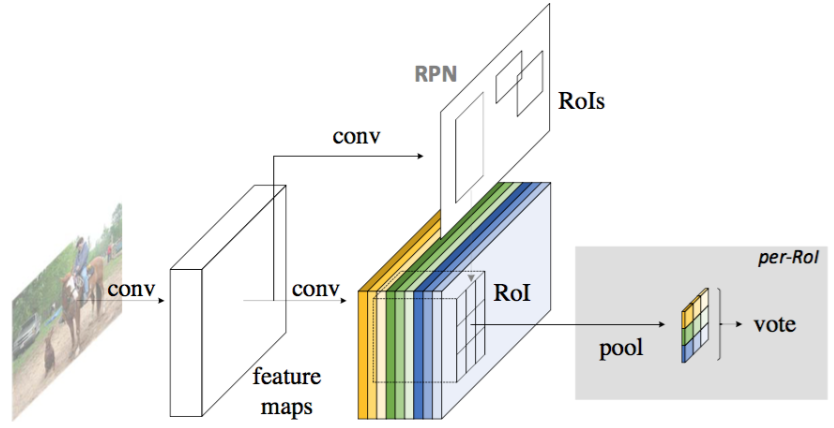

Figure 2: Overall architecture of R-FCN. A Region Proposal Network (RPN) [18] proposes candidate RoIs, which (RoIs)are then applied on the score maps. All learnable weight layers are convolutional and are computed on the entire image; the per-RoI computational cost is negligible（忽略不计）.
Given the proposal regions (RoIs), the R-FCN architecture is designed to classify the RoIs into object categories and background. In R-FCN, all learnable weight layers are convolutional and are computed on the entire image. The last convolutional layer produces a bank of position-sensitive score maps for each category, and thus has a -channel output layer with C object categories (+1 for background). The bank of score maps correspond to a k×k spatial grid describing relative positions. For example, with k×k=3×3, the 9 score maps encode the cases of {top-left, top-center, top-right, …, bottom-right} of an object category.
our position-sensitive RoI layer conducts selective pooling, and each of the k×k bin aggregates responses from only one score map out of the bank of k×k score maps.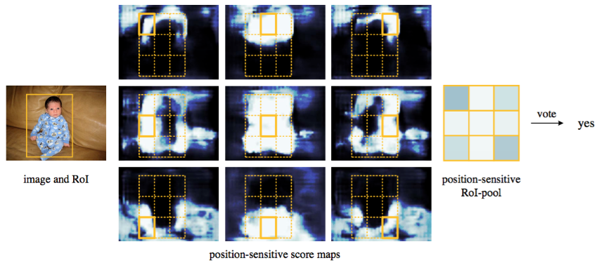

Figure 3: Visualization of R-FCN (k × k = 3 × 3) for the person category.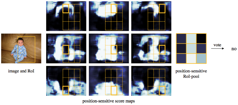

Figure 4: Visualization when an RoI does not correctly overlap the object.
Backbone architecture. The incarnation of R-FCN in this paper is based on ResNet-101 [9].We remove the average pooling layer and the fc layer and only use the convolutional layers to compute feature maps. The last convolutional block in ResNet-101 is 2048-d, and we attach a randomly initialized 1024-d 1×1 convolutional layer for reducing dimension (to be precise, this increases the depth in Table 1 by 1). Then we apply the -channel convolutional layer to generate score maps, as introduced next.