Faster R-CNN:
Towards Real-Time Object Detection with Region Proposal Networks
1. Introduction
RPNs are designed to efficiently predict region proposals with a wide range of scales and aspect ratios. In contrast to prevalent methods [8], [9], [1], [2] that use pyramids of images (Figure 1, a) or pyramids of filters (Figure 1, b), we introduce novel “anchor” boxes that serve as references at multiple scales and aspect ratios. Our scheme can be thought of as a pyramid of regression references (Figure 1, c), which avoids enumerating images or filters of multiple scales or aspect ratios. This model performs well when trained and tested using single-scale images and thus benefits running speed.
RPN被设计为使用具有不同尺度和长宽比的区域有效预测候选区域。与使用图像金字塔(图1,a)或滤波器金字塔(图1,b)的流行方法[8],[9],[1]相比,我们引入新的“锚”盒作为多种尺度和长宽比的参考。我们的方案可以被认为是回归引用金字塔(图1,c),它避免了枚举多种比例或长宽比的图像或滤波器。这个模型在使用单尺度图像进行训练和测试时运行良好,从而有利于运行速度。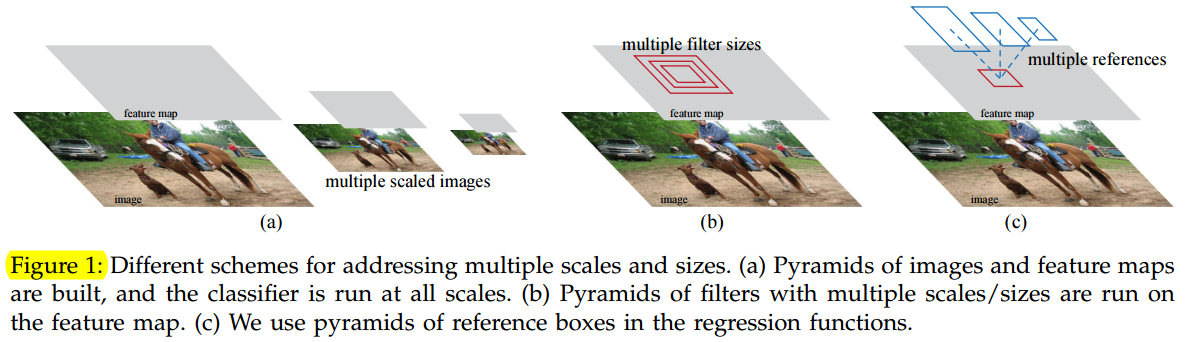
To unify RPNs with Fast R-CNN [2] object detection networks, we propose a training scheme that alternates between fine-tuning for the region proposal task and then fine-tuning for object detection, while keeping the proposals fixed. This scheme converges quickly and produces a unified network with convolutional features that are shared between both tasks.
为了将RPN与Fast R-CNN 2]目标检测网络相结合,我们提出了一种训练方案(交替训练),在微调候选区域任务和微调目标检测之间进行交替,交替时保持候选区域的固定。该方案快速收敛,并产生两个任务之间共享卷积特征的统一网络。
the frameworks of RPN and Faster R-CNN have been adopted and generalized to other methods, such as 3D object detection [13], part-based detection [14], instance segmentation [15], and image captioning [16].
RPN和Faster R-CNN的框架已经被采用并推广到其他方法,如3D目标检测[13],基于部件的检测[14],实例分割[15]和图像说明[16]。
2. RELATED WORK
Object proposal methods were adopted as external modules independent of the detectors (e.g., Selective Search [4] object detectors, R-CNN [5], and Fast R-CNN [2]).
目标候选区域方法被当成一个外部模块使用,它是独立于检测器的(例如,选择性搜索[4]目标检测器,R-CNN[5]和Fast R-CNN[2])。
3. FASTER R-CNN
Our object detection system, called Faster R-CNN, is composed of two modules. The first module is a deep fully convolutional network that proposes regions, and the second module is the Fast R-CNN detector [2] that uses the proposed regions. The entire system is a single, unified network for object detection (Figure 2). Using the recently popular terminology of neural networks with attention [31] mechanisms, the RPN module tells the Fast R-CNN module where to look.
我们的目标检测系统,称为Faster R-CNN,由两个模块组成。第一个模块是用于生成候选区域的深度全卷积网络,第二个模块是使用这些候选区域的Fast R-CNN检测器[2]。整个系统是一个单个的,统一的目标检测网络(图2)。使用最近流行的“注意力”机制的神经网络术语,RPN模块告诉Fast R-CNN模块应该往哪里看(往候选区域看)。
3.1 Region Proposal Networks
A Region Proposal Network (RPN) takes an image (of any size) as input and outputs a set of rectangular object proposals, each with an objectness score.Because our ultimate goal is to share computation with a Fast R-CNN object detection network [2], we assume that both nets share a common set of convolutional layers. In our experiments, we investigate the Zeiler and Fergus model 32, which has 5 shareable convolutional layers and the Simonyan and Zisserman model 3, which has 13 shareable convolutional layers.
区域生成网络(RPN):
输入:任意大小的图像。
输出:一组矩形的目标候选区域,每个区域都有一个目标得分。
我们的最终目标是与Fast R-CNN目标检测网络[2]共享计算,所以我们假设两个网络共享一组共同的卷积层。在我们的实验中,我们研究了具有5个共享卷积层的Zeiler和Fergus模型[32](ZF)和具有13个共享卷积层的Simonyan和Zisserman模型[3]。
To generate region proposals, we slide a small network over the convolutional feature map output by the last shared convolutional layer. This small network takes as input an n×nspatial window of the input convolutional feature map. Each sliding window is mapped to a lower-dimensional feature (256-d for ZF and 512-d for VGG, with ReLU [33] following). This feature is fed into two sibling fully-connected layers——a box-regression layer (reg) and a box-classification layer (cls). We use n=3 in this paper, noting that the effective receptive field on the input image is large (171 and 228 pixels for ZF and VGG, respectively). This mini-network is illustrated at a single position in Figure 3 (left). Note that because the mini-network operates in a sliding-window fashion, the fully-connected layers are shared across all spatial locations. This architecture is naturally implemented with an n×n convolutional layer followed by two sibling 1 × 1 convolutional layers (for reg and cls, respectively).
为了生成候选区域,我们在最后的共享卷积层输出的卷积特征映射上滑动一个小网络(滑动窗口)。这个小网络将输入卷积特征映射的n×n空间窗口作为输入。每个滑动窗口映射到一个低维特征(ZF为256维,VGG为512维,后面是ReLU[33])。这个低维特征被输入到两个子全连接层——一个边界框回归层(reg)和一个边界框分类层(cls)。在本文中,我们使用n=3,注意输入图像上的有效感受野是大的(ZF和VGG分别为171和228个像素)。图3(左)显示了这个小型网络的一个位置。请注意,因为小网络以滑动窗口方式运行,所有空间位置共享全连接层。这种架构通过一个n×n卷积层,后面接着两个子1×1卷积层(分别用于reg和cls)自然地实现。
3.1.1 Anchors
At each sliding-window location, we simultaneously predict multiple region proposals, where the number of maximum possible proposals for each location is denoted as k. So the reg layer has 4k outputs encoding the coordinates of k boxes, and the cls layer outputs 2k scores that estimate probability of object or not object for each proposal. The k proposals are parameterized relative to k reference boxes, which we call anchors. An anchor is centered at the sliding window in question, and is associated with a scale and aspect ratio (Figure 3, left). By default we use 3 scales and 3 aspect ratios, yielding k=9 anchors at each sliding position. For a convolutional feature map of a size W × H (typically ∼2,400), there are WHk anchors in total.
在每个滑动窗口位置,我们同时预测多个候选区域,其中每个位置上最大可能区域的数目表示为k。因此,reg层具有4k个输出,编码k个边界框的坐标,cls层输出2k个分数,估计每个区域是目标或不是目标的概率。k个候选是参数化的。锚点位于所讨论的滑动窗口的中心,并与一个尺度和长宽比相关(图3左)。默认情况下,我们使用3个尺度和3个长宽比,在每个滑动位置产生k=9个锚点。对于大小为W×H(通常约为2400)的卷积特征映射,总共有WHk个锚点。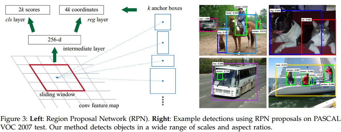
An important property of our approach is that it is translation invariant, both in terms of the anchors and the functions that compute proposals relative to the anchors. If one translates an object in an image, the proposal should translate and the same function should be able to predict the proposal in either location.
The translation-invariant property also reduces the model size. our method has a (4+2)×9-dimensional convolutional output layer in the case of k=9 anchors. As a result, our output layer has 2.8×10^4 parameters (512×(4+2)×9 for VGG-16).
我们的方法的一个重要特性是它是平移不变的,无论是在锚点还是计算相对于锚点的候选区域的函数。如果在图像中平移目标,候选区域也应该平移,并且同样的函数应该能够在任一位置预测候选区域。
平移不变特性也减小了模型的大小。我们的方法在k=9个锚点的情况下有(4+2)×9维的(RPN)卷积输出层。因此,我们的输出层具有2.8×10^4个参数(对于VGG-16为512×(4+2)×9)
Our design of anchors presents a novel scheme for addressing multiple scales (and aspect ratios). As shown in Figure 1, there have been two popular ways for multi-scale predictions. The first way is based on image/feature pyramids. The images are resized at multiple scales, and feature maps (HOG [8] or deep convolutional features [9], [1], [2]) are computed for each scale (Figure 1(a)). This way is often useful but is time-consuming. The second way is to use sliding windows of multiple scales (and/or aspect ratios) on the feature maps. If this way is used to address multiple scales, it can be thought of as a “pyramid of filters” (Figure 1(b)). The second way is usually adopted jointly with the first way [8].
our anchor-based method is built on a pyramid of anchors, which is more cost-efficient. Our method classifies and regresses bounding boxes with reference to anchor boxes of multiple scales and aspect ratios. It only relies on images and feature maps of a single scale, and uses filters (sliding windows on the feature map) of a single size. We show by experiments the effects of this scheme for addressing multiple scales and sizes (Table 8).
The design of multi-scale anchors is a key component for sharing features without extra cost for addressing scales.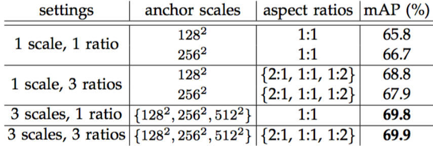
我们的锚点设计提出了一个新的方案来解决多尺度(和长宽比)。如图1所示,多尺度预测有两种流行的方法。第一种方法是基于图像/特征金字塔,图像在多个尺度上进行缩放,并且针对每个尺度(图1(a))计算特征映射(HOG[8]或深卷积特征[9],[1],[2])。这种方法通常是有用的,但是非常耗时。第二种方法是在特征映射上使用多尺度(和/或长宽比)的滑动窗口。如果用这种方法来解决多尺度问题,可以把它看作是一个“滤波器金字塔”(图1(b))。第二种方法通常与第一种方法联合采用[8]。
我们的基于锚点方法建立在锚点金字塔上,这是更具成本效益的。我们的方法参照多个不同大小和比例的锚点框对边界框进行分类和回归。它只依赖单一尺度的图像和特征映射,并使用单一尺寸的滤波器(特征映射上的滑动窗口)。我们通过实验来展示这个方案解决多尺度和尺寸的效果(表8)。
多尺度锚点设计是共享特征的关键组件,不需要额外的成本来处理尺度。
3.1.2 Loss Function
For training RPNs, we assign a binary class label (of being an object or not) to each anchor. We assign a positive label to two kinds of anchors: (i) the anchor/anchors with the highest Intersection-over-Union (IoU) overlap with a ground-truth box, or (ii) an anchor that has an IoU overlap higher than 0.7 with any ground-truth box. Note that a single ground-truth box may assign positive labels to multiple anchors. Usually the second condition is sufficient to determine the positive samples; but we still adopt the first condition for the reason that in some rare cases the second condition may find no positive sample. We assign a negative label to a non-positive anchor if its IoU ratio is lower than 0.3 for all ground-truth boxes. Anchors that are neither positive nor negative do not contribute to the training objective.
为了训练RPN,我们为每个锚点分配一个二值类别标签(是目标或不是目标)。我们给两种锚点分配一个正标签:(i)具有与某一个实际边界框的重叠最高交并比(IoU)的锚点,或者(ii)具有与任意一个实际边界框的重叠超过0.7 IoU的锚点。注意,单个真实边界框可以为多个锚点分配正标签。通常第二个条件足以确定正样本;但我们仍然采用第一个条件,因为在一些极少数情况下,第二个条件可能找不到正样本。对于所有的真实边界框,如果一个锚点的IoU比率低于0.3,我们给非正的锚点分配一个负标签。既不正面也不负面的锚点不会有助于训练目标函数。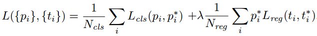
Here, i is the index of an anchor in a mini-batch and pipi is the predicted probability of anchor i being an object. The ground-truth label pi∗ is 1 if the anchor is positive, and is 0 if the anchor is negative. ti is a vector representing the 4 parameterized coordinates of the predicted bounding box, and ti∗ is that of the ground-truth box associated with a positive anchor. The classification loss Lcls is log loss over two classes (object vs not object). For the regression loss, we use Lreg(ti,t∗i)=R(ti−t∗i) where R is the robust loss function (smooth L1) defined in [2]. The term pi∗Lreg means the regression loss is activated only for positive anchors (pi∗=1) and is disabled otherwise (pi∗=0). The outputs of the cls and reg layers consist of pipi and ti respectively.
The two terms are normalized by Ncls and Nreg and weighted by a balancing parameter λ. In our current implementation (as in the released code), the clscls term in Eqn.(1) is normalized by the mini-batch size (ie, Ncls=256) and the regreg term is normalized by the number of anchor locations (ie, Nreg∼2,400). By default we set λ=10, and thus both cls and reg terms are roughly equally weighted. We show by experiments that the results are insensitive to the values of λin a wide range(Table 9). We also note that the normalization as above is not required and could be simplified. 是一个小批量数据中锚点的索引,
 是锚点作为目标的预测概率。如果锚点为正,真实标签
 ,如果锚点为负,则为
 。
。 是表示预测边界框4个参数化坐标的向量,而
 是与正锚点相关的真实GT边界框的向量。cls和reg层的输出分别由和组成。
分类损失Lcls是两个类别上(目标或不是目标)的对数损失。对于回归损失,我们使用 ,其中R是在[2]中定义的鲁棒损失函数(平滑L1)。项
 表示回归损失仅对于正锚点()激活。
Loss的两项用 和
和 进行标准化,并由一个平衡参数λ加权。在我们目前的实现中(如在发布的代码中),方程中的cls项通过小批量(mini-batch size)的大小(例如
 )进行归一化,reg项根据锚点的数量(即,
 )进行归一化。默认情况下,我们设置λ=10,因此cls和reg项的权重大致相等。我们通过实验显示,结果对λ在较大范围取值不敏感(表9)。我们还注意到,上面的归一化不是必需的,可以简化。
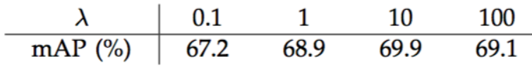
where x, y, w, and h denote the box’s center coordinates and its width and height. Variables x, xa, and x∗ are for the predicted box, anchor box, and ground-truth box respectively (likewise for y,w,h). This can be thought of as bounding-box regression from an anchor box to a nearby ground-truth box.
在对边框的回归校正中,我们采用以下4个坐标作为参数。其中, 表示边界框的中心坐标及其宽和高。变量
 分别表示预测边界框,锚点框(anchor box)和实际(ground-truth)边界框(
 也是一样的表示方法)。这可以被认为是从锚点框到邻近的实际边界框的回归。
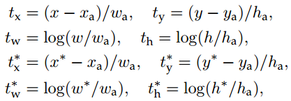
3.1.3 Training RPNs
The RPN can be trained end-to-end by back-propagation and stochastic gradient descent (SGD) [35]. We follow the “image-centric” sampling strategy from [2] to train this network. Each mini-batch arises from a single image that contains many positive and negative example anchors. It is possible to optimize for the loss functions of all anchors, but this will bias towards negative samples as they are dominate. Instead, we randomly sample 256 anchors in an image to compute the loss function of a mini-batch, where the sampled positive and negative anchors have a ratio of up to 1:1. If there are fewer than 128 positive samples in an image, we pad the mini-batch with negative ones.
RPN可以通过反向传播和随机梯度下降(SGD)进行端对端训练[35]。我们遵循[2]的“以图像为中心”的采样策略来训练这个网络。每个小批量数据都从包含许多正面和负面示例锚点的单张图像中产生。对所有锚点的损失函数进行优化是可能的,但是这样会偏向于负样本,因为它们是占主导地位的。取而代之的是,我们在一张图像中随机采样256个锚点,计算一个小批量数据的损失函数,其中采样的正锚点和负锚点的比率可达1:1。如果图像中的正样本少于128个,我们使用负样本填充小批量数据。
We randomly initialize all new layers by drawing weights from a zero-mean Gaussian distribution with standard deviation 0.01. All other layers (i.e., the shared convolutional layers) are initialized by pre-training a model for ImageNet classification [36], as is standard practice [5].
我们通过从标准差为0.01的零均值高斯分布中提取权重来随机初始化所有新层。所有其他层(即共享卷积层)通过预训练的ImageNet分类模型[36]来初始化,如同标准实践[5]。
3.2 Sharing Features for RPN and Fast R-CNN
Both RPN and Fast R-CNN, trained independently, will modify their convolutional layers in different ways. We therefore need to develop a technique that allows for sharing convolutional layers between the two networks, rather than learning two separate networks. We discuss three ways for training networks with features shared:
(i) Alternating training. In this solution, we first train RPN, and use the proposals to train Fast R-CNN. The network tuned by Fast R-CNN is then used to initialize RPN, and this process is iterated. This is the solution that is used in all experiments in this paper.
4-Step Alternating Training. In this paper, we adopt a pragmatic 4-step training algorithm to learn shared features via alternating optimization. In the first step, we train the RPN as described in Section 3.1.3. This network is initialized with an ImageNet-pre-trained model and fine-tuned end-to-end for the region proposal task. In the second step, we train a separate detection network by Fast R-CNN using the proposals generated by the step-1 RPN. This detection network is also initialized by the ImageNet-pre-trained model. At this point the two networks do not share convolutional layers. In the third step, we use the detector network to initialize RPN training, but we fix the shared convolutional layers and only fine-tune the layers unique to RPN. Now the two networks share convolutional layers. Finally, keeping the shared convolutional layers fixed, we fine-tune the unique layers of Fast R-CNN. As such, both networks share the same convolutional layers and form a unified network. A similar alternating training can be run for more iterations, but we have observed negligible improvements.
独立训练的RPN和Fast R-CNN将以不同的方式修改卷积层。因此,我们需要开发一种允许在两个网络之间共享卷积层的技术,而不是学习两个独立的网络。我们讨论三个方法来训练具有共享特征的网络:
(一)交替训练。在这个解决方案中,我们首先训练RPN,并使用(生成的)区域来训练Fast R-CNN。由Fast R-CNN微调的网络然后被用于初始化RPN,并且重复这个过程。这是本文所有实验中使用的解决方案。
四步交替训练。在本文中,我们采用实用的四步训练算法,通过交替优化学习共享特征。在第一步中,我们按照3.1.3节的描述训练RPN。该网络使用ImageNet的预训练模型进行初始化,并针对区域生成任务进行了端到端的微调。在第二步中,我们使用由第一步RPN生成的区域,由Fast R-CNN训练单独的检测网络。该检测网络也由ImageNet的预训练模型进行初始化。此时两个网络不共享卷积层。在第三步中,我们使用检测器网络来初始化RPN训练,但是我们固定共享的卷积层,并且只对RPN特有的层进行微调。现在这两个网络共享卷积层。最后,保持共享卷积层的固定,我们对Fast R-CNN的独有层进行微调。于是,两个网络共享相同的卷积层并形成统一的网络。类似的交替训练可以运行更多的迭代,但是我们只观察到可以忽略的改进。
3.3 Implementation Details
During training, we ignore all cross-boundary anchors so they do not contribute to the loss. For a typical 1000×600 image, there will be roughly 20000 (≈60×40×9) anchors in total. With the cross-boundary anchors ignored, there are about 6000 anchors per image for training. If the boundary-crossing outliers are not ignored in training, they introduce large, difficult to correct error terms in the objective, and training does not converge. During testing, however, we still apply the fully convolutional RPN to the entire image. This may generate cross-boundary proposal boxes, which we clip to the image boundary.
Some RPN proposals highly overlap with each other. To reduce redundancy, we adopt non-maximum suppression (NMS) on the proposal regions based on their cls scores. We fix the IoU threshold for NMS at 0.7, which leaves us about 2000 proposal regions per image. As we will show, NMS does not harm the ultimate detection accuracy, but substantially reduces the number of proposals. After NMS, we use the top-N ranked proposal regions for detection. In the following, we train Fast R-CNN using 2000 RPN proposals, but evaluate different numbers of proposals at test-time.
在训练过程中,我们忽略了所有的跨界锚点,所以不会造成损失。对于一个典型的1000×600的图片,总共将会有大约20000(≈60×40×9)个锚点(框)。跨界锚点被忽略,每张图像约有6000个锚点用于训练。如果跨界异常值在训练中不被忽略,则会在目标函数中引入大的,难以纠正的误差项,且训练不会收敛。但在测试过程中,我们仍然将全卷积RPN应用于整张图像。这可能会产生跨边界的边界框,对这些边框我们沿着图像边界进行裁剪。
一些RPN生成区域互相之间高度重叠。为了减少冗余,我们根据他们的cls分数采取非极大值抑制(NMS)。我们将NMS的IoU阈值固定为0.7,这就给每张图像留下了大约2000个区域。正如我们将要展示的那样,NMS不会损害最终的检测准确性,但会大大减少生成区域的数量。在NMS之后,我们使用前N个区域来进行检测。接下来,我们使用2000个RPN生成区域对Fast R-CNN进行训练,但在测试时评估不同数量的区域。
4. EXPERIMENTS
The plots show that the RPN method behaves gracefully when the number of proposals drops from 2000 to 300. This explains why the RPN has a good ultimate detection mAP when using as few as 300 proposals. As we analyzed before, this property is mainly attributed to the cls term of the RPN.
从图中可以看出,当候选区域数量从2000个减少到300个时,RPN方法表现优雅。这就解释了为什么RPN在使用300个区域时具有良好的最终检测mAP。正如我们之前分析过的,这个属性主要归因于RPN的cls项。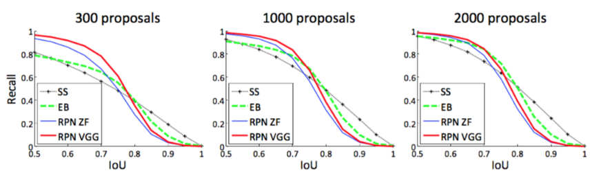

若有收获,就点个赞吧
0 人点赞
