2019年5月20日作者:SUNITANAYAK发表 评论
最近PyTorch因其使用和学习简单而获得了很多人的欢迎。特斯拉AI高级总监Andrej Karpathy在他的推文中说了以下内容。
抛开笑话,PyTorch也非常透明,可以帮助研究人员和数据科学家实现高生产率。
此博客是以下系列的一部分:
| PyTorch初学者 |
|---|
| PyTorch for Beginners:基础知识 |
| PyTorch for Beginners:使用预训练模型进行图像分类 |
| PyTorch中使用迁移学习的图像分类 |
| 使用ONNX和Caffe2进行PyTorch模型推理 |
| PyTorch for Beginners:使用torchvision进行语义分割 |
| 物体检测 |
| 人体姿势关键点检测 |
在这篇文章中,我们描述了如何在PyTorch中进行图像分类。我们将使用CalTech256)数据集的一个子集对10种不同动物的图像进行分类。我们将讨论数据集准备,数据扩充以及构建分类器的步骤。我们使用迁移学习来使用由预训练模型ResNet50学习的边缘,纹理等低级图像特征,然后训练我们的分类器来学习我们的数据集图像中的更高级别的细节,如眼睛,腿等.ResNet50已经被在ImageNet上训练了数百万张图片。
我们与完整的代码共享一个python笔记本,并在这篇文章中分享重要的片段,以便读者能够理解它是如何工作的。
下载代码要轻松学习本教程,请单击下面的按钮下载代码。免费!
下载代码
虽然我们试图使博客文章自给自足,但我们仍然鼓励读者在进一步开展之前熟悉Pytorch的基础知识。
数据集准备
该 CalTech256数据集有分为256个不同的标记类与其他“混乱”类沿30607倍的图像。
训练整个数据集需要数小时,因此我们将研究包含10种动物的数据集的子集 - 熊,黑猩猩,长颈鹿,大猩猩,美洲驼,鸵鸟,豪猪,臭鼬,三角龙和斑马。这样我们就可以更快地进行实验 然后,代码也可用于训练整个数据集。
这些文件夹中的图像数量从81(对于臭鼬)到212(对于大猩猩)不等。我们使用这些类别中的前60个图像进行训练,接下来的10个图像用于验证,其余用于下面的实验中的测试。
最后我们有600张训练图像,100张验证图像,409张测试图像和10类动物。
如果您想复制实验,请按照以下步骤操作
- 下载 CalTech256 数据集
- 使用名称train,valid和test创建三个目录 。
- 在列车和测试目录中创建10个子目录。子目录应该命名为熊,黑猩猩,长颈鹿,大猩猩,美洲驼,鸵鸟,豪猪,臭鼬,三角龙和斑马。
- 将Caltech256数据集中的前60张图像移动到目录train/bear,并为每只动物重复此操作。
- 将接下来的10张图像在Caltech256数据集中移动到目录valid/bear,并为每只动物重复此操作。
- 将剩余的熊图像(即未包含在列车或有效文件夹中的图像)复制到目录test/bear。对每只动物重复这个。
数据扩充
可以通过多种方式修改可用训练集中的图像以在训练过程中包含更多变化,使得训练的模型变得更加通用并且在不同类型的测试数据上表现良好。输入数据也可以有多种尺寸。在将批量数据一起用于训练之前,需要将它们标准化为固定大小和格式。
每个输入图像首先通过许多变换。我们尝试通过在转换中引入一些随机性来插入一些变体。在每个时期中,对每个图像应用单组变换。当我们训练多个时期时,模型可以看到输入图像的更多变化,每个时期的变换具有新的随机变化。这导致数据增加,然后模型尝试概括更多。
下面我们看到Triceratops图像的转换版本的示例。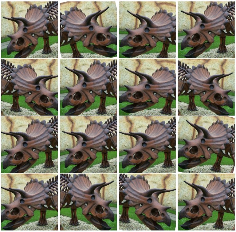
三角龙图像的转换版本
让我们回顾一下我们用于数据扩充的转换。
变换RandomResizedCrop以随机大小裁剪输入图像(在原始大小的0.8到1.0的范围内,以及在0.75到1.33的默认范围内的随机宽高比)。然后将裁剪大小调整为256×256。
RandomRotation将图像旋转一个在-15到15度之间随机选择的角度。
RandomHorizontalFlip水平地随机翻转图像,默认概率为50%。
CenterCrop从中心裁剪出一张224×224的图像。
ToTensor将具有0-255范围内值的PIL图像转换为浮点Tensor,并将它们除以255,将它们归一化到0-1的范围。
标准化采用3通道张量,并通过通道的输入平均值和标准偏差对每个通道进行标准化。平均和标准偏差矢量作为3个元素矢量输入。张量中的每个通道归一化为T =(T - mean)/(标准差)
所有上述转换都使用Compose链接在一起。
# Applying Transforms to the Dataimage_transforms = {'train': transforms.Compose([transforms.RandomResizedCrop(size=256, scale=(0.8, 1.0)),transforms.RandomRotation(degrees=15),transforms.RandomHorizontalFlip(),transforms.CenterCrop(size=224),transforms.ToTensor(),transforms.Normalize([0.485, 0.456, 0.406],[0.229, 0.224, 0.225])]),'valid': transforms.Compose([transforms.Resize(size=256),transforms.CenterCrop(size=224),transforms.ToTensor(),transforms.Normalize([0.485, 0.456, 0.406],[0.229, 0.224, 0.225])]),'test': transforms.Compose([transforms.Resize(size=256),transforms.CenterCrop(size=224),transforms.ToTensor(),transforms.Normalize([0.485, 0.456, 0.406],[0.229, 0.224, 0.225])])}
请注意,对于验证和测试数据,我们不执行RandomResizedCrop,RandomRotation和RandomHorizontalFlip转换。相反,我们只是将验证图像的大小调整为256×256并裁剪出中心224×224,以便能够将它们与预训练模型一起使用。然后将图像转换为张量,并通过ImageNet中所有图像的均值和标准偏差进行归一化。
数据加载
接下来,让我们看看如何使用上面定义的转换并加载要用于训练的数据。
Image Classification using Transfer Learning in PyTorchMAY 20, 2019 BY SUNITA NAYAK LEAVE A COMMENTImage Classification ResultsRecently PyTorch has gained a lot of popularity because of its simplicity to use and learn. Andrej Karpathy, Senior Director of AI at Tesla, said the following in his tweet.Putting jokes aside, PyTorch is also very transparent and can help researchers and data scientists achieve high productivity.This blog is part of the following series:PyTorch for BeginnersPyTorch for Beginners: BasicsPyTorch for Beginners: Image Classification using Pre-trained modelsImage Classification using Transfer Learning in PyTorchPyTorch Model Inference using ONNX and Caffe2PyTorch for Beginners: Semantic Segmentation using torchvisionObject DetectionHuman Pose Keypoint DetectionIn this post, we describe how to do image classification in PyTorch.We will use a subset of the CalTech256 dataset to classify images of 10 different kinds of animals. We will go over the dataset preparation, data augmentation and then steps to build the classifier. We use transfer learning to use the low level image features like edges, textures etc. learnt by a pretrained model, ResNet50, and then train our classifier to learn the higher level details in our dataset images like eyes, legs etc. ResNet50 has already been trained on ImageNet with millions of images.We share a python notebook with the complete code and share important snippets in this post so that the reader can understand how it works.Download Code To easily follow along this tutorial, please download code by clicking on the button below. It's FREE!DOWNLOAD CODEWhile we have tried to make the blog post self sufficient,we still encourage the readers to get familiarized to the basics of Pytorch before proceeding further.Dataset PreparationThe CalTech256 dataset has 30,607 images categorized into 256 different labeled classes along with another ‘clutter’ class.Training the whole dataset will take hours, so we will work on a subset of the dataset containing 10 animals – bear, chimp, giraffe, gorilla, llama, ostrich, porcupine, skunk, triceratops and zebra. That way we can experiment faster. The code can then be used to train the whole dataset too.The number of images in these folders varies from 81(for skunk) to 212(for gorilla). We use the first 60 images in each of these categories for training, the next 10 images for validation and the rest for testing in our experiments below.So finally we have 600 training images, 100 validation images, 409 test images and 10 classes of animals.If you want to replicate the experiments, please follow the steps belowDownload the CalTech256 datasetCreate three directories with names train, valid and test.Create 10 sub-directories each inside the train and the test directories. The sub-directories should be named bear, chimp, giraffe, gorilla, llama, ostrich, porcupine, skunk, triceratops and zebra.Move the first 60 images for bear in the Caltech256 dataset to the directory train/bear, and repeat this for every animal.Move the next 10 images for bear in the Caltech256 dataset to the directory valid/bear, and repeat this for every animal.Copy the remaining images for bear (i.e. the ones not included in train or valid folders) to the directory test/bear. Repeat this for every animal.Data AugmentationThe images in the available training set can be modified in a number of ways to incorporate more variations in the training process, so that the trained model gets more generalized and performs well on different kinds of test data. Also the input data can come in a variety of sizes. They need to be normalized to a fixed size and format before batches of data are used together for training.Each of the input images are first passed through a number of transformations. We try to insert some variations by introducing some randomness into the transformations. In each epoch, a single set of transformations are applied to each image. When we train for multiple epochs, the models gets to see more variations of the input images with a new randomized variation of the transformation in each epoch. This results in data augmentation and the model then tries to generalize more.Below we see examples of the transformed versions of a Triceratops image.Data AugmentationTransformed versions of a Triceratops imageLet us go over the transformations we used for our data augmentation.The transform RandomResizedCrop crops the input image by a random size(within a scale range of 0.8 to 1.0 of the original size and a random aspect ratio in the default range of 0.75 to 1.33 ). The crop is then resized to 256×256.RandomRotation rotates the image by an angle randomly chosen between -15 to 15 degrees.RandomHorizontalFlip randomly flips the image horizontally with a default probability of 50%.CenterCrop crops an 224×224 image from the center.ToTensor converts the PIL Image which has values in the range of 0-255 to a floating point Tensor and normalizes them to a range of 0-1, by dividing it by 255.Normalize takes in a 3 channel Tensor and normalizes each channel by the input mean and standard deviation for the channel. Mean and standard deviation vectors are input as 3 element vectors. Each channel in the tensor is normalized as T = (T – mean)/(standard deviation)All the above transformations are chained together using Compose.# Applying Transforms to the Dataimage_transforms = {'train': transforms.Compose([transforms.RandomResizedCrop(size=256, scale=(0.8, 1.0)),transforms.RandomRotation(degrees=15),transforms.RandomHorizontalFlip(),transforms.CenterCrop(size=224),transforms.ToTensor(),transforms.Normalize([0.485, 0.456, 0.406],[0.229, 0.224, 0.225])]),'valid': transforms.Compose([transforms.Resize(size=256),transforms.CenterCrop(size=224),transforms.ToTensor(),transforms.Normalize([0.485, 0.456, 0.406],[0.229, 0.224, 0.225])]),'test': transforms.Compose([transforms.Resize(size=256),transforms.CenterCrop(size=224),transforms.ToTensor(),transforms.Normalize([0.485, 0.456, 0.406],[0.229, 0.224, 0.225])])}Note that for the validation and test data, we do not do the RandomResizedCrop, RandomRotation and RandomHorizontalFlip transformations. Instead, we just resize the validation images to 256×256 and crop out the center 224×224 in order to be able to use them with the pretrained model. Then the image is transformed into a tensor and normalized by the mean and standard deviation of all images in ImageNet.Data LoadingNext, let us see how to use the above defined transformations and load the data to be used for training.# Load the Data# Set train and valid directory pathstrain_directory = 'train'valid_directory = 'test'# Batch sizebs = 32# Number of classesnum_classes = 10# Load Data from foldersdata = {'train': datasets.ImageFolder(root=train_directory, transform=image_transforms['train']),'valid': datasets.ImageFolder(root=valid_directory, transform=image_transforms['valid']),'test': datasets.ImageFolder(root=test_directory, transform=image_transforms['test'])}# Size of Data, to be used for calculating Average Loss and Accuracytrain_data_size = len(data['train'])valid_data_size = len(data['valid'])test_data_size = len(data['test'])# Create iterators for the Data loaded using DataLoader moduletrain_data = DataLoader(data['train'], batch_size=bs, shuffle=True)valid_data = DataLoader(data['valid'], batch_size=bs, shuffle=True)test_data = DataLoader(data['test'], batch_size=bs, shuffle=True)# Print the train, validation and test set data sizestrain_data_size, valid_data_size, test_data_size
我们首先设置列车和验证数据目录,以及批量大小。然后我们使用DataLoader加载它们。请注意,我们之前讨论过的图像转换在使用DataLoader加载数据时应用于数据。数据的顺序也被洗牌。torchvision.transforms包和DataLoader是非常重要的PyTorch功能,使数据扩充和加载过程非常容易。
迁移学习
收集属于感兴趣的域的图像并从头开始训练分类器是非常困难和耗时的。因此,我们使用预先训练的模型作为基础并更改最后几层,以便我们可以根据我们期望的类对图像进行分类。这有助于我们即使使用小型数据集也能获得良好的结果,因为已经在预先训练的模型中从像ImageNet这样的更大的数据集中学习了基本的图像特征。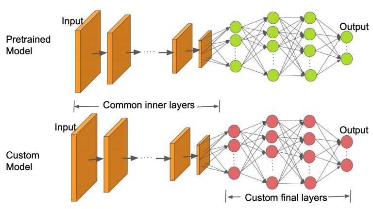
正如我们在上面的图像中看到的那样,内层与预训练模型保持相同,只更改最终层以适合我们的类数。在这项工作中,我们使用预先训练的ResNet50模型。
# Load pretrained ResNet50 Modelresnet50 ``= models.resnet50(pretrained``=``True``) |
|---|
Canziani等人列出了许多用于各种实际应用的预训练模型,分析了所获得的精度以及每个模型所需的推理时间。ResNet50是精确度和推理时间之间具有良好折衷的那些之一。在PyTorch中加载模型时,默认情况下其所有参数的’ requires_grad ‘字段都设置为true。这意味着将存储对参数值的每个改变,以便在用于训练的反向传播图中使用。这增加了内存需求。因此,由于我们已经训练过预训练模型中的大多数参数,因此我们将requires_grad字段重置为false。
# Freeze model parametersfor param in resnet50.parameters():param.requires_grad = False
然后我们用一小组Sequential层替换ResNet50模型的最后一层。ResNet50的最后一个完全连接层的输入被馈送到具有256个输出的线性层,然后将其馈送到ReLU和Dropout层。然后是256×10线性层,其具有10个输出,对应于我们的CalTech子集中的10个类。
由于我们将在GPU上进行训练,因此我们可以为GPU准备好模型。
# Convert model to be used on GPUresnet50 ``= resnet50.to(``'cuda:0'``) |
|---|
接下来,我们定义损失函数和用于训练的优化器。PyTorch提供多种损失功能。我们使用负损失似然函数,因为它可用于分类多个类。PyTorch还支持多个优化器。我们使用Adam优化器。Adam是最受欢迎的优化器之一,因为它可以单独调整每个参数的学习率。
# Define Optimizer and Loss Functionloss_func = nn.NLLLoss()optimizer = optim.Adam(resnet50.parameters())
训练
完整的训练代码在python笔记本中,但我们在这里提出了主要概念。对一组固定的时期进行训练,在一个时期内处理每个图像一次。训练数据加载器批量加载数据。在我们的例子中,我们给出了批量大小为32,这意味着每个批次最多可以有32个图像。
对于每个批次,输入图像通过模型,即前向传递,以获得输出。然后使用提供的loss_criterion或cost函数来计算使用地面实况和计算输出的损失。使用后向函数计算相对于可训练参数的损失梯度。请注意,对于迁移学习,我们只需要为属于模型末尾少数新添加的层的一小组参数计算梯度。对模型的汇总函数调用可以揭示实际参数数量和可训练参数的数量。正如我们在下面看到的,我们现在只需要训练模型参数总数的十分之一左右。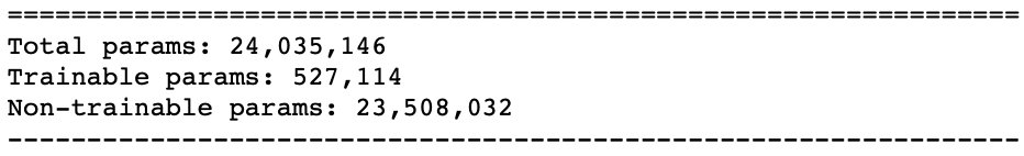
使用自动编程和反向传播完成梯度计算,使用链式法则在图中进行区分。PyTorch在后向传递中累积所有渐变。因此,必须在训练循环开始时将它们归零。这是使用优化器的zero_grad函数实现的。最后,在向后传递中计算梯度之后,使用优化器的步进函数更新参数。
计算整个批次的总损失和准确度,然后对所有批次进行平均,以获得整个时期的损失和准确度值。
for epoch in range(epochs):epoch_start = time.time()print("Epoch: {}/{}".format(epoch+1, epochs))# Set to training modemodel.train()# Loss and Accuracy within the epochtrain_loss = 0.0train_acc = 0.0valid_loss = 0.0valid_acc = 0.0for i, (inputs, labels) in enumerate(train_data_loader):inputs = inputs.to(device)labels = labels.to(device)# Clean existing gradientsoptimizer.zero_grad()# Forward pass - compute outputs on input data using the modeloutputs = model(inputs)# Compute lossloss = loss_criterion(outputs, labels)# Backpropagate the gradientsloss.backward()# Update the parametersoptimizer.step()# Compute the total loss for the batch and add it to train_losstrain_loss += loss.item() * inputs.size(0)# Compute the accuracyret, predictions = torch.max(outputs.data, 1)correct_counts = predictions.eq(labels.data.view_as(predictions))# Convert correct_counts to float and then compute the meanacc = torch.mean(correct_counts.type(torch.FloatTensor))# Compute total accuracy in the whole batch and add to train_acctrain_acc += acc.item() * inputs.size(0)print("Batch number: {:03d}, Training: Loss: {:.4f}, Accuracy: {:.4f}".format(i, loss.item(), acc.item()))
验证
随着对更多数量的时期进行训练,该模型倾向于过度拟合数据,导致其在新测试数据上的不良性能。保持单独的验证集很重要,这样我们就可以在正确的位置停止训练并防止过度拟合。在训练循环之后立即在每个时期进行验证。由于我们在验证过程中不需要任何梯度计算,因此它在torch.no_grad()块中完成。
对于每个验证批次,输入和标签将传输到GPU(如果cuda可用,则为cpu)。输入通过前向传递,然后是整个时期的批次和循环结束时的损失和精度计算。
# Validation - No gradient tracking neededwith torch.no_grad():# Set to evaluation modemodel.eval()# Validation loopfor j, (inputs, labels) in enumerate(valid_data_loader):inputs = inputs.to(device)labels = labels.to(device)# Forward pass - compute outputs on input data using the modeloutputs = model(inputs)# Compute lossloss = loss_criterion(outputs, labels)# Compute the total loss for the batch and add it to valid_lossvalid_loss += loss.item() * inputs.size(0)# Calculate validation accuracyret, predictions = torch.max(outputs.data, 1)correct_counts = predictions.eq(labels.data.view_as(predictions))# Convert correct_counts to float and then compute the meanacc = torch.mean(correct_counts.type(torch.FloatTensor))# Compute total accuracy in the whole batch and add to valid_accvalid_acc += acc.item() * inputs.size(0)print("Validation Batch number: {:03d}, Validation: Loss: {:.4f}, Accuracy: {:.4f}".format(j, loss.item(), acc.item()))# Find average training loss and training accuracyavg_train_loss = train_loss/train_data_sizeavg_train_acc = train_acc/float(train_data_size)# Find average training loss and training accuracyavg_valid_loss = valid_loss/valid_data_sizeavg_valid_acc = valid_acc/float(valid_data_size)history.append([avg_train_loss, avg_valid_loss, avg_train_acc, avg_valid_acc])epoch_end = time.time()print("Epoch : {:03d}, Training: Loss: {:.4f}, Accuracy: {:.4f}%, \n\t\tValidation : Loss : {:.4f}, Accuracy: {:.4f}%, Time: {:.4f}s".format(epoch, avg_train_loss, avg_train_acc*100, avg_valid_loss, avg_valid_acc*100, epoch_end-epoch_start))
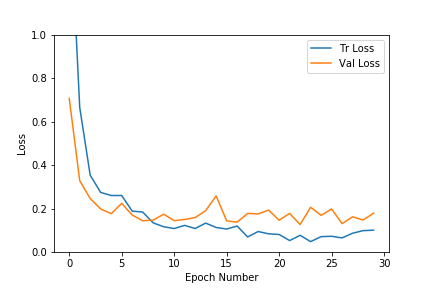
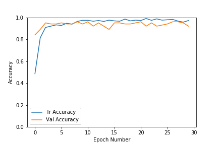
正如我们在上面的图中所看到的,对于该数据集,验证和训练损失都很快得到了解决。精确度也会非常快地增加到0.9的范围。随着时代数量的增加,训练损失不断减少,导致过度拟合,但验证结果并没有大幅提高。因此我们选择了具有更高精度和更低损耗的时代模型。如果我们提前停止也是更好的,以防止过度拟合训练数据。在我们的例子中,我们选择了#8时期,其验证准确度为96%。
在早期停止过程也可以自动完成。一旦损失低于给定阈值,我们就可以停止,并且对于给定的一组时期,验证准确性不会提高。
推理
一旦我们有了模型,我们就可以对各个测试图像或整个测试数据集进行推断,以获得测试精度。测试集精度计算与验证代码类似,不同之处在于它是在测试数据集上执行的。我们在Python笔记本中包含了函数computeTestSetAccuracy。让我们看下面如何找到给定测试图像的输出类。
输入图像首先经历用于验证/测试数据的所有变换。然后将得到的张量转换为4维张量,并通过模型,该模型输出不同类别的对数概率。模型输出的指数为我们提供了类概率,然后我们选择概率最高的类作为输出类。
选择概率最高的类作为输出类。
def predict(model, test_image_name):transform = image_transforms['test']test_image = Image.open(test_image_name)plt.imshow(test_image)test_image_tensor = transform(test_image)if torch.cuda.is_available():test_image_tensor = test_image_tensor.view(1, 3, 224, 224).cuda()else:test_image_tensor = test_image_tensor.view(1, 3, 224, 224)with torch.no_grad():model.eval()# Model outputs log probabilitiesout = model(test_image_tensor)ps = torch.exp(out)topk, topclass = ps.topk(1, dim=1)print("Output class : ", idx_to_class[topclass.cpu().numpy()[0][0]])
在具有409个图像的测试集上实现了92.4%的准确度。
以下是未在训练或验证中使用的新测试数据的一些分类结果。具有概率分数的图像的最高预测类别覆盖在右上角。如下所示,以最高概率预测的类通常是正确的。还要注意,具有第二高概率的类在外观上与其他9个类中的其余类别中的实际类通常是最接近的动物。
我们刚刚看到了如何使用经过训练的1000个ImageNet类的预训练模型,可以非常有效地对属于我们感兴趣的10个不同类别的图像进行分类。
我们在一个小数据集上显示了分类结果。在以后的文章中,我们将在更难的数据集上应用相同的迁移学习方法来解决更难的现实问题。敬请关注 !
承认
我感谢我们的实习生Kushashwa Ravi Shrimali撰写了这篇文章的部分代码。
参考

若有收获,就点个赞吧
0 人点赞
