在PyTorch中构建Faster RCNN的指南

介绍
- 特征提取
锚箱
Region Proposal Network.
生成提供Fast R-CNN网络的提议
提案目标
Fast R-CNN
损失函数
RPN Loss
Fast R-CNN损失

介绍

Faster R-CNN是第一个完全适用于深度学习的框架之一。它建立在Fast RCNN的基础之上，它确实建立在RCNN和SPP-Net的思想基础之上。虽然我们在构建Faster RCNN框架时带来了一些Fast RCNN的想法，但我们不会详细讨论这些框架。其中一个原因是Faster R-CNN表现非常好，并且它不使用传统的计算机视觉技术，如选择性搜索等。在很高的层次上，Fast RCNN和Faster RCNN的工作原理如下面的流程图所示。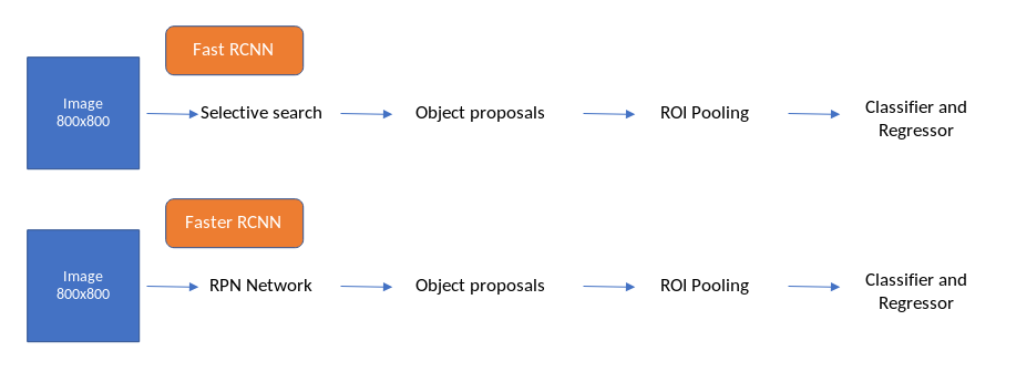

我们已经写了一个详细的博客帖子上的物体检测框架这里。这将成为那些希望通过自己编码来理解Faster RCNN的人的指南。
您可以在上图中看到的唯一区别是，Faster RCNN已经用RPN(区域提议网络)网络取代了选择性搜索。选择性搜索算法使用SIFT和HOG描述符来生成对象提议，并且在CPU上每个图像需要2秒。这是一个昂贵的过程，Fast RCNN总共需要2.3秒才能在一个图像上生成预测，即使使用VGGnet等非常深的图像分类器(现在也使用ResNet和ResNext)，Fast RCNN也能以5 FPS(每秒帧数)工作。 )在后端。

<—more—>
因此，为了从头开始构建Faster RCNN，我们需要清楚地理解以下四个主题，

[Flow]

Region Proposal network (RPN)
RPN loss functions
Region of Interest Pooling (ROI)
ROI loss functions

Region Proposal网络还引入了一种名为Anchor boxes的新概念，在构建对象检测管道之后，它已经成为一种金标准。让我们深入了解并了解管道的各个阶段如何在Faster RCNN中协同工作。
在训练网络时，Faster R-CNN中的通常数据流如下所示：

功能从图像中提取。
创建锚点目标。
来自RPN网络的位置和对象得分预测。
取来自aka proposal layer的前N个位置及其对象分数
通过Fast R-CNN网络传递这些前N个位置，并在4中建议为每个位置生成位置和cls预测。
为4中建议的每个位置生成提案目标
使用2和3来计算rpn_cls_loss和rpn_reg_loss。
使用5和6来计算roi_cls_loss和roi_reg_loss。

我们将配置VGG16并将其用作本实验的后端。注意，我们可以以类似的方式使用任何标准分类网络。

特征提取

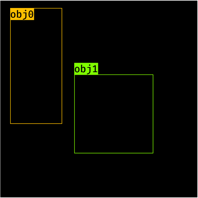
我们从图像和一组边界框开始，以及下面定义的标签。

import torch
image = torch.zeros((1, 3, 800, 800)).float()
bbox = torch.FloatTensor([[20, 30, 400, 500], [300, 400, 500, 600]]) # [y1, x1, y2, x2] format
labels = torch.LongTensor([6, 8]) # 0 represents background
sub_sample = 16

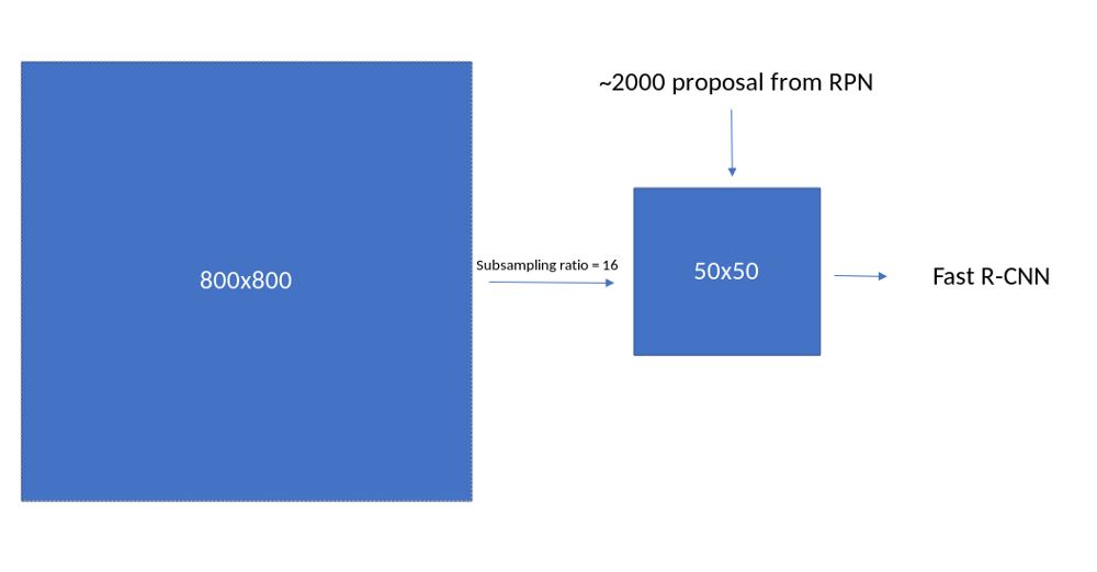
VGG16网络在此用作特征提取模块，它充当RPN网络和Fast_R-CNN网络的骨干网。我们需要对VGG网络进行一些更改才能使其工作。由于网络的输入是800，因此特征提取模块的输出应具有(800//16)的特征映射大小。因此，我们需要检查VGG16模块在哪里实现此功能映射大小，并修剪网络直到der。这可以通过以下方式完成。

创建一个虚拟图像并将volatile设置为False
列出vgg16的所有图层
当图像的output_size(特征映射)低于所需级别(800//16)时，将图像传递通过图层并对列表进行子集化
将此列表转换为Sequential模块。

让我们看看每一步

创建一个虚拟图像并将volatile设置为False。

import torchvision
dummy_img = torch.zeros((1, 3, 800, 800)).float()
print(dummy_img)
#Out: torch.Size([1, 3, 800, 800])

2.列出VGG16的所有层。

model = torchvision.models.vgg16(pretrained=True)
fe = list(model.features)
print(fe) # length is 15
# [Conv2d(3, 64, kernel_size=(3, 3), stride=(1, 1), padding=(1, 1)),
#  ReLU(inplace),
#  Conv2d(64, 64, kernel_size=(3, 3), stride=(1, 1), padding=(1, 1)),
#  ReLU(inplace),
#  MaxPool2d(kernel_size=(2, 2), stride=(2, 2), dilation=(1, 1), ceil_mode=False),
#  Conv2d(64, 128, kernel_size=(3, 3), stride=(1, 1), padding=(1, 1)),
#  ReLU(inplace),
#  Conv2d(128, 128, kernel_size=(3, 3), stride=(1, 1), padding=(1, 1)),
#  ReLU(inplace),
#  MaxPool2d(kernel_size=(2, 2), stride=(2, 2), dilation=(1, 1), ceil_mode=False),
#  Conv2d(128, 256, kernel_size=(3, 3), stride=(1, 1), padding=(1, 1)),
#  ReLU(inplace),
#  Conv2d(256, 256, kernel_size=(3, 3), stride=(1, 1), padding=(1, 1)),
#  ReLU(inplace),
#  Conv2d(256, 256, kernel_size=(3, 3), stride=(1, 1), padding=(1, 1)),
#  ReLU(inplace),
#  MaxPool2d(kernel_size=(2, 2), stride=(2, 2), dilation=(1, 1), ceil_mode=False),
#  Conv2d(256, 512, kernel_size=(3, 3), stride=(1, 1), padding=(1, 1)),
#  ReLU(inplace),
#  Conv2d(512, 512, kernel_size=(3, 3), stride=(1, 1), padding=(1, 1)),
#  ReLU(inplace),
#  Conv2d(512, 512, kernel_size=(3, 3), stride=(1, 1), padding=(1, 1)),
#  ReLU(inplace),
#  MaxPool2d(kernel_size=(2, 2), stride=(2, 2), dilation=(1, 1), ceil_mode=False),
#  Conv2d(512, 512, kernel_size=(3, 3), stride=(1, 1), padding=(1, 1)),
#  ReLU(inplace),
#  Conv2d(512, 512, kernel_size=(3, 3), stride=(1, 1), padding=(1, 1)),
#  ReLU(inplace),
#  Conv2d(512, 512, kernel_size=(3, 3), stride=(1, 1), padding=(1, 1)),
#  ReLU(inplace),
#  MaxPool2d(kernel_size=(2, 2), stride=(2, 2), dilation=(1, 1), ceil_mode=False)]

3.将图像传递到图层并检查您获得此尺寸的位置。

req_features = []
k = dummy_img.clone()
for i in fe:
    k = i(k)
    if k.size()[2] < 800//16:
        break
    fee.append(i)
    out_channels = k.size()[1]
print(len(req_features)) #30
print(out_channels) # 512

4.将此列表转换为Sequential模块。

faster_rcnn_fe_extractor = nn.Sequential(*req_features)

现在这个faster_rcnn_fe_extractor可以用作我们的后端。让我们计算一下这些功能

out_map = faster_rcnn_fe_extractor（image）
print（out_map.size（））
#Out：torch.Size（[1,512,50,50]）

锚箱

这是我们第一次遇到锚箱。对锚箱的详细了解将使我们能够非常容易地理解物体检测。因此，让我们详细谈谈如何做到这一点。

在特征图位置生成锚点
在所有特征图位置生成锚点。
将对象的标签和位置(相对于锚点)分配给每个锚点。
在特征图位置生成锚点

我们将使用8,16,32的anchor_scales，0.5,1,2的比率和16的子采样(因为我们将图像从800 px汇集到50px)。现在，输出特征图中的每个像素都映射到图像中对应的16 * 16像素。如下图所示

图像到特征图映射

我们需要首先在这个16 * 16像素的顶部生成锚框，并且类似地沿着x轴和y轴生成锚框以获得所有锚框。这在步骤2中完成。
在特征图上的每个像素位置，我们需要生成9个锚框(anchor_scales的数量和比率的数量)，并且每个锚框将具有’y1’，’x1’，’y2’，’x2’。因此，在每个位置，锚将具有(9,4)的形状。让我们从一个填充零值的空数组开始。

import numpy as np
ratio = [0.5, 1, 2]
anchor_scales = [8, 16, 32]
anchor_base = np.zeros((len(ratios) * len(scales), 4), dtype=np.float32)
print(anchor_base)
#Out:
# array([[0., 0., 0., 0.],
#        [0., 0., 0., 0.],
#        [0., 0., 0., 0.],
#        [0., 0., 0., 0.],
#        [0., 0., 0., 0.],
#        [0., 0., 0., 0.],
#        [0., 0., 0., 0.],
#        [0., 0., 0., 0.],
#        [0., 0., 0., 0.]], dtype=float32)

让与对应填充这些值y1，x1，y2，x2在每个anchor_scale和比率。我们这个基地锚的中心将在

ctr_y = sub_sample / 2.
ctr_x = sub_sample / 2.
print(ctr_y, ctr_x)
# Out: (8, 8)
for i in range(len(ratios)):
  for j in range(len(anchor_scales)):
    h = sub_sample * anchor_scales[j] * np.sqrt(ratios[i])
    w = sub_sample * anchor_scales[j] * np.sqrt(1./ ratios[i])
    index = i * len(anchor_scales) + j
    anchor_base[index, 0] = ctr_y - h / 2.
    anchor_base[index, 1] = ctr_x - w / 2.
    anchor_base[index, 2] = ctr_y + h / 2.
    anchor_base[index, 3] = ctr_x + w / 2.
#Out:
# array([[ -37.254833,  -82.50967 ,   53.254833,   98.50967 ],
#        [ -82.50967 , -173.01933 ,   98.50967 ,  189.01933 ],
#        [-173.01933 , -354.03867 ,  189.01933 ,  370.03867 ],
#        [ -56.      ,  -56.      ,   72.      ,   72.      ],
#        [-120.      , -120.      ,  136.      ,  136.      ],
#        [-248.      , -248.      ,  264.      ,  264.      ],
#        [ -82.50967 ,  -37.254833,   98.50967 ,   53.254833],
#        [-173.01933 ,  -82.50967 ,  189.01933 ,   98.50967 ],
#        [-354.03867 , -173.01933 ,  370.03867 ,  189.01933 ]],
#       dtype=float32)

这些是第一个特征映射像素的锚点位置，我们现在必须在特征映射的所有位置生成这些锚点。还要注意，负值意味着锚框在图像维度之外。在后面的部分中，我们将使用-1标记它们，并在计算丢失函数和生成锚框提议时将其删除。此外，由于我们在每个位置都有9个锚点，并且在图像中有50 50个这样的位置，我们总共会获得17500(50 50 * 9)个锚点。让我们现在生成其他锚点，
2.在所有特征图位置生成锚点。
为了做到这一点，我们需要首先为每个特征映射像素生成中心。

fe_size = (800//16)
ctr_x = np.arange(16, (fe_size+1) * 16, 16)
ctr_y = np.arange(16, (fe_size+1) * 16, 16)

循环通过ctr_x和ctr_y将为我们提供每个位置的中心。sudo代码如下

For x in shift_x:
  For y in shift_y:
    Generate anchors at (x, y) locations

在下面可以看到相同的情况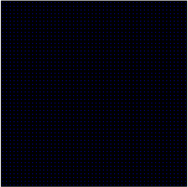

锚点以图像为中心
让我们使用python生成这个中心

index = 0
for x in range(len(ctr_x)):
    for y in range(len(ctr_y)):
        ctr[index, 1] = ctr_x[x] - 8
        ctr[index, 0] = ctr_y[y] - 8
        index +=1

输出将是每个位置的(x，y)值，如上图所示。我们一起拥有2500个锚定中心。现在在每个中心我们需要生成锚箱。这可以使用我们用于在一个位置生成锚点的代码来完成，为每个锚点的供应中心添加一个for循环提取。让我们看看这是如何完成的。

anchors = np.zeros((fe_size * fe_size * 9), 4)
index = 0
for c in ctr:
  ctr_y, ctr_x = c
  for i in range(len(ratios)):
    for j in range(len(anchor_scales)):
      h = sub_sample * anchor_scales[j] * np.sqrt(ratios[i])
      w = sub_sample * anchor_scales[j] * np.sqrt(1./ ratios[i])
      anchors[index, 0] = ctr_y - h / 2.
      anchors[index, 1] = ctr_x - w / 2.
      anchors[index, 2] = ctr_y + h / 2.
      anchors[index, 3] = ctr_x + w / 2.
      index += 1
print(anchors.shape)
#Out: [22500, 4]

注意：为了简单起见，我使这段代码看起来非常冗长。有更好的方法来生成锚箱。
这些将成为我们将进一步使用的图像的最终锚点。让我们直观地了解这些锚点如何在图像上展开

锚箱(400,400)

图像的有效锚框

将对象的标签和位置(相对于锚点)分配给每个锚点。

既然我们已经生成了所有的锚框，我们需要查看图像中的对象并将它们分配给包含它们的特定锚框。Faster_R-CNN有一些指导方针可以为锚箱分配标签
我们为两种锚点分配一个正面标签a)具有最高交叉点(IoU)的锚点/锚点与地面真值框重叠或b)具有地面的IoU重叠高于0.7的锚点-truth框。
请注意，单个地面实况对象可以将正标签分配给多个锚点。
c)如果所有地面实况框的IoU比率低于0.3，我们为非正锚定分配负标签。d)既不是正面也不是否定的锚点对培训目标没有贡献。
让我们看看这是如何完成的。

bbox = np.asarray([[20, 30, 400, 500], [300, 400, 500, 600]], dtype=np.float32) # [y1, x1, y2, x2] format
labels = np.asarray([6, 8], dtype=np.int8) # 0 represents background

我们将通过以下方式为锚箱分配标签和位置。

找到有效锚框的索引并使用这些索引创建一个数组。创建一个标签数组，其形状索引数组填充-1。
检查天气上述条件之一a，b，c是否满意，并相应填写标签。包含正锚箱(标签为1)，注意哪个基础真实对象导致了这个。
计算与锚箱相关联的地面实况的位置(loc)到锚箱。
对于所有无效的锚框和我们为所有有效锚箱计算的值，通过填充-1来重新组织所有锚框。
输出应该是带有(N，1)数组的标签和带有(N，4)数组的loc。
找到所有有效锚箱的索引。

index_inside = np.where(
        (anchors[:, 0] >= 0) &
        (anchors[:, 1] >= 0) &
        (anchors[:, 2] <= 800) &
        (anchors[:, 3] <= 800)
    )[0]
print(index_inside.shape)
#Out: (8940,)

使用inside_index形状创建一个空标签数组并填充-1。默认设置为(d)

label = np.empty((len(inside_index), ), dtype=np.int32)
 label.fill(-1)
 print(label.shape)
#Out = (8940, )

创建一个包含有效锚框的数组

valid_anchor_boxes = anchors[inside_index]
print(valid_anchor_boxes.shape)
#Out = (8940, 4)

对于每个有效的锚箱，计算每个地面实况对象的iou。由于我们有8940个锚箱和2个地面实况对象，我们应该得到一个带有(8490,2)的数组作为输出。在两个方框之间计算你的sudo代码将是

- Find the max of x1 and y1 in both the boxes (xn1, yn1)
- Find the min of x2 and y2 in both the boxes (xn2, yn2)
- Now both the boxes are intersecting only
 if (xn1 < xn2) and (yn2 < yn1)
      - iou_area will be (xn2 - xn1) * (yn2 - yn1)
 else
      - iuo_area will be 0
- similarly calculate area for anchor box and ground truth object
- iou = iou_area/(anchor_box_area + ground_truth_area - iou_area)

用于计算ious的python代码如下

ious = np.empty((len(valid_anchors), 2), dtype=np.float32)
ious.fill(0)
print(bbox)
for num1, i in enumerate(valid_anchors):
    ya1, xa1, ya2, xa2 = i  
    anchor_area = (ya2 - ya1) * (xa2 - xa1)
    for num2, j in enumerate(bbox):
        yb1, xb1, yb2, xb2 = j
        box_area = (yb2- yb1) * (xb2 - xb1)
        inter_x1 = max([xb1, xa1])
        inter_y1 = max([yb1, ya1])
        inter_x2 = min([xb2, xa2])
        inter_y2 = min([yb2, ya2])
        if (inter_x1 < inter_x2) and (inter_y1 < inter_y2):
            iter_area = (inter_y2 - inter_y1) * \
(inter_x2 - inter_x1)
            iou = iter_area / \
(anchor_area+ box_area - iter_area)            
        else:
            iou = 0.
        ious[num1, num2] = iou
print(ious.shape)
#Out: [22500, 2]

注意：使用numpy数组，可以更有效地完成这些计算，并且使用更少的详细信息。但是我试着以这种方式留在这里，这样没有强代数的人也能理解。
考虑到a和b的情景，我们需要在这里找到两件事

每个gt_box及其相应锚点的最高iou
每个锚箱及其相应的地面实况框中最高的iou

case-1

gt_argmax_ious = ious.argmax(axis=0)
print(gt_argmax_ious)
gt_max_ious = ious[gt_argmax_ious, np.arange(ious.shape[1])]
print(gt_max_ious)
# Out:
# [2262 5620]
# [0.68130493 0.61035156]

case-2

argmax_ious = ious.argmax（axis = 1）
print（argmax_ious.shape）
print（argmax_ious）
max_ious = ious [np.arange（len（inside_index）），argmax_ious] 
print（max_ious）#out 
：
＃（22500，）＃[0,1,0 
，...，
1,0,0 ] ＃[0.06811669 0.07083762 0.07083762 ... 0. 0. 0.]

找到具有此max_ious(gt_max_ious)的anchor_boxes

gt_argmax_ious = np.where(ious == gt_max_ious)[0]
print(gt_argmax_ious)
# Out:
# [2262, 2508, 5620, 5628, 5636, 5644, 5866, 5874, 5882, 5890, 6112,
#        6120, 6128, 6136, 6358, 6366, 6374, 6382]

现在我们有三个数组

argmax_ious - 告诉每个锚点哪个基础事实对象最大。
max_ious - 用每个锚告诉max_iou和地面实况对象。
gt_argmax_ious - 告诉具有最高交叉点(IoU)重叠的锚点与地面实况框重叠。

使用argmax_ious和max_ious，我们可以为锚点框分配标签和位置，以满足[b]和[c]。使用gt_argmax_ious，我们可以为锚点框分配标签和位置，以满足[a]。
让我们把阈值放在一些变量上

pos_iou_threshold  = 0.7
neg_iou_threshold = 0.3

将否定标签(0)分配给max_iou小于负阈值的所有锚框[E]

label[max_ious < neg_iou_threshold] = 0

将正标签(1)分配给所有与地面实况框具有最高IoU重叠的锚箱[a]

label[gt_argmax_ious] = 1

将正标签(1)分配给max_iou大于正阈值的所有锚箱[b]

label [max_ious> = pos_iou_threshold] = 1

Training RPN The Faster_R-CNN paper phrases as follows Each mini-batch arises from a single image that contains many positive and negitive example anchors, but this will bias towards negitive samples as they are dominate. Instead, we randomly sample 256 anchors in an image to compute the loss function of a mini-batch, where the sampled positive and negative anchors have a ratio of up to 1:1. If there are fewer than 128 positive samples in an image, we pad the mini-batch with negitive ones.. From this we can derive two variable as follows

pos_ratio = 0.5 
n_sample = 256

总阳性样本

n_pos = pos_ratio * n_sample

现在我们需要从正标签中随机抽取n_pos个样本，然后忽略(-1)剩余的样本。在某些情况下，我们得到的n_pos样本少于n_pos样本，因为我们将随机抽样(n_sample - n_pos)负样本(0)并将忽略标签分配给剩余的锚框。这是使用以下代码完成的。

阳性样本

pos_index = np.where(label == 1)[0]
if len(pos_index) > n_pos:
    disable_index = np.random.choice(pos_index, size=(len(pos_index) - n_pos), replace=False)
    label[disable_index] = -1

负面样本

n_neg = n_sample * np.sum(label == 1)
neg_index = np.where(label == 0)[0]
if len(neg_index) > n_neg:
    disable_index = np.random.choice(neg_index, size=(len(neg_index) - n_neg), replace = False)
    label[disable_index] = -1

将位置分配给锚箱
现在，我们可以使用具有最大iou的地面实况对象为每个锚箱分配位置。注意，我们将锚定位置分配给所有有效的锚定框而不管其标记，稍后当我们计算损失时，我们可以使用简单的过滤器删除它们。
我们已经知道哪个地面实况对象与每个锚箱有很高的关系，现在我们需要找到关于锚箱位置的地面实况的位置。Faster_R-CNN为此使用以下参数

t_{x} = (x - x_{a})/w_{a}
t_{y} = (y - y_{a})/h_{a}
t_{w} = log(w/ w_a)
t_{h} = log(h/ h_a)

x，y，w，h是实心框中心坐标，宽度和高度。x_a，y_a，h_a和w_a以及锚箱中心cooridinates，宽度和高度。

对于每个锚框，找到具有max_iou的groundtruth对象

max_iou_bbox = bbox[argmax_ious]
print(max_iou_bbox)
#Out
# [[ 20.,  30., 400., 500.],
#  [ 20.,  30., 400., 500.],
#  [ 20.,  30., 400., 500.],
#  ...,
#  [ 20.,  30., 400., 500.],
#  [ 20.,  30., 400., 500.],
#  [ 20.,  30., 400., 500.]]

为了找到t {x}，t {y}，t {w}，t {h}，我们需要将有效锚箱和相关地面实况框的y1，x1，y2，x2格式与max iou转换为ctr_y ，ctr_x，h，w格式。

height = valid_anchors[:, 2] - valid_anchors[:, 0]
width = valid_anchors[:, 3] - valid_anchors[:, 1]
ctr_y = valid_anchors[:, 0] + 0.5 * height
ctr_x = valid_anchors[:, 1] + 0.5 * width
base_height = max_iou_bbox[:, 2] - max_iou_bbox[:, 0]
base_width = max_iou_bbox[:, 3] - max_iou_bbox[:, 1]
base_ctr_y = max_iou_bbox[:, 0] + 0.5 * base_height
base_ctr_x = max_iou_bbox[:, 1] + 0.5 * base_width

使用上面的公式来查找loc

eps = np.finfo(height.dtype).eps
height = np.maximum(height, eps)
width = np.maximum(width, eps)
dy = (base_ctr_y - ctr_y) / height
dx = (base_ctr_x - ctr_x) / width
dh = np.log(base_height / height)
dw = np.log(base_width / width)
anchor_locs = np.vstack((dy, dx, dh, dw)).transpose()
print(anchor_locs)
#Out:
# [[ 0.5855727   2.3091455   0.7415673   1.647276  ]
#  [ 0.49718437  2.3091455   0.7415673   1.647276  ]
#  [ 0.40879607  2.3091455   0.7415673   1.647276  ]
#  ...
#  [-2.50802    -5.292254    0.7415677   1.6472763 ]
#  [-2.5964084  -5.292254    0.7415677   1.6472763 ]
#  [-2.6847968  -5.292254    0.7415677   1.6472763 ]]

现在我们得到了与每个有效锚箱相关联的anchor_locs和label

让我们使用inside_index变量将它们映射到原始锚点。使用-1(忽略)填充无效的锚框标签，使用0填充位置。

最终标签：

anchor_labels = np.empty（（len（anchors），），dtype = label.dtype）
anchor_labels.fill（-1）
anchor_labels [inside_index] = label

最终位置

anchor_locations = np.empty((len(anchors),) + anchors.shape[1:], dtype=anchor_locs.dtype)
anchor_locations.fill(0)
anchor_locations[inside_index, :] = anchor_locs

最后两个矩阵是

anchor_locations [N，4] - [22500,4]
anchor_labels [N，] - [22500]

这些用作RPN网络的目标。我们将在下一节中看到如何设计此RPN网络。

Region Proposal Network.

正如我们之前所讨论的，在此工作之前，使用选择性搜索，CPMC，MCG，边缘框等生成网络的区域提议.Faster_R-CNN是使用深度学习来演示生成区域提议的第一项工作。

RPN网络

网络包含一个卷积模块，在其上面将有一个回归层，用于预测锚点内盒子的位置
为了生成区域提议，我们在我们在特征提取模块中获得的卷积特征映射输出上滑动一个小网络。该小网络将输入卷积特征映射的n×n空间窗口作为输入。每个滑动窗口都映射到较低维度的特征[512个特征]。此功能被送入两个兄弟完全连接的层

A box regrression layer
A box classification layer

我们使用n = 3，如Faster_R-CNN论文中所述。我们可以使用nxn卷积层，然后是两个sibiling 1 x 1卷积层来实现此架构

import torch.nn as nn
mid_channels = 512
in_channels = 512 # depends on the output feature map. in vgg 16 it is equal to 512
n_anchor = 9 # Number of anchors at each location
conv1 = nn.Conv2d(in_channels, mid_channels, 3, 1, 1)
reg_layer = nn.Conv2d(mid_channels, n_anchor *4, 1, 1, 0)
cls_layer = nn.Conv2d(mid_channels, n_anchor *2, 1, 1, 0) 
## I will be going to use softmax here. you can equally use sigmoid if u replace 2 with 1.

该论文告诉他们用零均值和0.01标准差初始化这些层的权重和基数的零。让我们这样做

# conv sliding layer
conv1.weight.data.normal_(0, 0.01)
conv1.bias.data.zero_()
# Regression layer
reg_layer.weight.data.normal_(0, 0.01)
reg_layer.bias.data.zero_()
# classification layer
cls_layer.weight.data.normal_(0, 0.01)
cls_layer.bias.data.zero_()

现在，我们在特征提取状态下得到的输出应该被发送到该网络，以预测对象的位置以及与其相关的对象性得分。

x = conv1(out_map) # out_map is obtained in section 1
pred_anchor_locs = reg_layer(x)
pred_cls_scores = cls_layer(x)
print(pred_cls_scores.shape, pred_anchor_locs.shape)
#Out:
#torch.Size([1, 18, 50, 50]) torch.Size([1, 36, 50, 50])

让我们重新格式化这些并使其与我们之前设计的锚定目标对齐。我们还将找到每个锚框的对象性分数，因为这用于提案层，我们将在下一节中讨论

pred_anchor_locs = pred_anchor_locs.permute(0, 2, 3, 1).contiguous().view(1, -1, 4)
print(pred_anchor_locs.shape)
#Out: torch.Size([1, 22500, 4])
pred_cls_scores = pred_cls_scores.permute(0, 2, 3, 1).contiguous()
print(pred_cls_scores)
#Out torch.Size([1, 50, 50, 18])
objectness_score = pred_cls_scores.view(1, 50, 50, 9, 2)[:, :, :, :, 1].contiguous().view(1, -1)
print(objectness_score.shape)
#Out torch.Size([1, 22500])
pred_cls_scores  = pred_cls_scores.view(1, -1, 2)
print(pred_cls_scores.shape)
# Out torch.size([1, 22500, 2])

我们完成了部分

pred_cls_scores和pred_anchor_locs是RPN网络的输出和更新权重的损失
pred_cls_scores和objectness_scores用作提议层的输入，其生成一组提议，这些提议将被RoI网络进一步使用。我们将在下一节中看到这一点。

生成提供Fast R-CNN网络的提议
提案功能将采用以下参数
Weather training_mode or testing mode
nms_thresh
n_train_pre_nms — number of bboxes before nms during training
n_train_post_nms — number of bboxes after nms during training
n_test_pre_nms — number of bboxes before nms during testing
n_test_post_nms — number of bboxes after nms during testing
min_size — minimum height of the object required to create a proposal.

Faster R_CNN说，RPN提案彼此高度重叠。为了减少冗余，我们根据其cls分数对提议区域采用非最大抑制(NMS)。我们将NMS的IoU阈值修正为0.7，这使得每个图像大约有2000个提议区域。在消融研究之后，作者表明NMS不会损害最终的检测准确性，但会大大减少提案的数量。在NMS之后，我们使用排名前N的提议区域进行检测。在下文中，我们使用2000个RPN提议训练Fast R-CNN。在测试过程中，他们仅评估了300个提案，他们已经使用不同的数字对此进行了测

nms_thresh = 0.7
n_train_pre_nms = 12000
n_train_post_nms = 2000
n_test_pre_nms = 6000
n_test_post_nms = 300
min_size = 16

我们需要做以下事情来为网络生成感兴趣区域提案。

将loc预测从rpn网络转换为bbox [y1，x1，y2，x2]格式。
将预测的框剪辑到图像
删除高度或宽度<threshold(min_size)的预测框。
按分数从最高到最低对所有(提案，分数)对进行排序。
取顶部pre_nms_topN(例如训练时为12000，测试时为300)。
应用nms阈值> 0.7
取顶部pos_nms_topN(例如训练时为2000，测试时为300)

我们将查看本节其余部分中的每个阶段

将loc预测从rpn网络转换为bbox [y1，x1，y2，x2]格式。

这是我们在将基础事实分配给锚箱时所做的相反操作。该操作通过取消参数化和对图像的偏离来解码预测。公式如下

x = (w_{a} * ctr_x_{p}) + ctr_x_{a}
y = (h_{a} * ctr_x_{p}) + ctr_x_{a}
h = np.exp(h_{p}) * h_{a}
w = np.exp(w_{p}) * w_{a}
and later convert to y1, x1, y2, x2 format

将锚点格式从y1，x1，y2，x2转换为ctr_x，ctr_y，h，w

anc_height = anchors[:, 2] - anchors[:, 0]
anc_width = anchors[:, 3] - anchors[:, 1]
anc_ctr_y = anchors[:, 0] + 0.5 * anc_height
anc_ctr_x = anchors[:, 1] + 0.5 * anc_width

使用上面的公式转换预测位置。在此之前，转换pred_anchor_locs和objectness_score到numpy的阵列

pred_anchor_locs_numpy = pred_anchor_locs[0].data.numpy()
objectness_score_numpy = objectness_score[0].data.numpy()
dy = pred_anchor_locs_numpy[:, 0::4]
dx = pred_anchor_locs_numpy[:, 1::4]
dh = pred_anchor_locs_numpy[: 2::4]
dw = pred_anchor_locs_numpy[: 3::4]
ctr_y = dy * anc_height[:, np.newaxis] + anc_ctr_y[:, np.newaxis]
ctr_x = dx * anc_width[:, np.newaxis] + anc_ctr_x[:, np.newaxis]
h = np.exp(dh) * anc_height[:, np.newaxis]
w = np.exp(dw) * anc_width[:, np.newaxis]

将[ctr_x，ctr_y，h，w]转换为[y1，x1，y2，x2]格式

roi = np.zeros(pred_anchor_locs_numpy.shape, dtype=loc.dtype)
roi[:, 0::4] = ctr_y - 0.5 * h
roi[:, 1::4] = ctr_x - 0.5 * w
roi[:, 2::4] = ctr_y + 0.5 * h
roi[:, 3::4] = ctr_x + 0.5 * w
#Out:
# [[ -36.897102,  -80.29519 ,   54.09939 ,  100.40507 ],
#  [ -83.12463 , -165.74298 ,   98.67854 ,  188.6116  ],
#  [-170.7821  , -378.22214 ,  196.20844 ,  349.81198 ],
#  ...,
#  [ 696.17816 ,  747.13306 ,  883.4582  ,  836.77747 ],
#  [ 621.42114 ,  703.0614  ,  973.04626 ,  885.31226 ],
#  [ 432.86267 ,  622.48926 , 1146.7059  ,  982.9209  ]]

将预测的框剪辑到图像

img_size = (800, 800) #Image size
roi[:, slice(0, 4, 2)] = np.clip(
            roi[:, slice(0, 4, 2)], 0, img_size[0])
roi[:, slice(1, 4, 2)] = np.clip(
    roi[:, slice(1, 4, 2)], 0, img_size[1])
print(roi)
#Out:
# [[  0.     ,   0.     ,  54.09939, 100.40507],
#  [  0.     ,   0.     ,  98.67854, 188.6116 ],
#  [  0.     ,   0.     , 196.20844, 349.81198],
#  ...,
#  [696.17816, 747.13306, 800.     , 800.     ],
#  [621.42114, 703.0614 , 800.     , 800.     ],
#  [432.86267, 622.48926, 800.     , 800.     ]]

删除高度或宽度<阈值的预测框。

hs = roi[:, 2] - roi[:, 0]
ws = roi[:, 3] - roi[:, 1]
keep = np.where((hs >= min_size) & (ws >= min_size))[0]
roi = roi[keep, :]
score = objectness_score_numpy[keep]
print(score.shape)
#Out:
##(22500, ) all the boxes have minimum size of 16

按分数从最高到最低对所有(提案，分数)对进行排序。

order = score.ravel().argsort()[::-1]
print(order)
#Out:
#[ 889,  929, 1316, ...,  462,  454,    4]

取得最高的pre_nms_topN(例如训练时为12000，测试时为300)

order = order[:n_train_pre_nms]
roi = roi[order, :]
print(roi.shape)
print(roi)
#Out
# (12000, 4)
# [[607.93866,   0.     , 800.     , 113.38187],
#  [  0.     ,   0.     , 235.29704, 369.64795],
#  [572.177  ,   0.     , 800.     , 373.0086 ],
#  ...,
#  [250.07968, 186.61633, 434.6356 , 276.70615],
#  [490.07974, 154.6163 , 674.6356 , 244.70615],
#  [266.07968, 602.61633, 450.6356 , 692.7062 ]]

应用非最大抑制阈值> 0.7

第一个问题，什么是非最大抑制？这是我们删除/合并极高重叠边界框的过程。如果我们看下面的图表，有很多重叠的边界框，我们想要一些独特的边界框，并且不会重叠太多。我们将门槛保持在0.7。阈值定义合并/删除重叠边界框所需的最小重叠区域

NMS的sudo代码以下列方式工作

- Take all the roi boxes [roi_array]
- Find the areas of all the boxes [roi_area]
- Take the indexes of order the probability score in descending order [order_array]
keep = []
while order_array.size > 0:
  - take the first element in order_array and append that to keep  
  - Find the area with all other boxes
  - Find the index of all the boxes which have high overlap with this box
  - Remove them from order array
  - Iterate this till we get the order_size to zero (while loop)
- Ouput the keep variable which tells what indexes to consider.

取顶部pos_nms_topN(例如训练时为2000，测试时为300)

y1 = roi[:, 0]
x1 = roi[:, 1]
y2 = roi[:, 2]
x2 = roi[:, 3]
area = (x2 - x1 + 1) * (y2 - y1 + 1)
order = scores.argsort()[::-1]
keep = []
while order.size > 0
    i = order[0]
    xx1 = np.maximum(x1[i], x1[order[1:]])
    yy1 = np.maximum(y1[i], y1[order[1:]])
    xx2 = np.minimum(x2[i], x2[order[1:]])
    yy2 = np.minimum(y2[i], y2[order[1:]])
    w = np.maximum(0.0, xx2 - xx1 + 1)
    h = np.maximum(0.0, yy2 - yy1 + 1)
    inter = w * h
    ovr = inter / (areas[i] + areas[order[1:]] - inter)
    inds = np.where(ovr <= thresh)[0]
    order = order[inds + 1]
keep = keep[:n_train_post_nms] # while training/testing , use accordingly
roi = roi[keep] # the final region proposals

获得最终区域提议，这被用作Fast_R-CNN对象的输入，其最终尝试预测对象位置(关于所提议的框)和对象的类(每个提议的分类)。首先，我们研究如何为这些网络的培训创建目标。之后，我们将研究如何实现这个Fast 的r-cnn网络，并将这些提议传递给网络以获得预测的输出。然后，我们将确定损失，我们将计算rpn损失和Fast r-cnn损失。

提案目标

Fast R-CNN网络采用区域提议(从前一节中的提议层获得)，地面实况框及其各自的标签作为输入。它将采用以下参数

n_sample：从roi中采样的样本数，默认值为128。
pos_ratio：n_samples中的正例数。默认值为0.25。
pos_iou_thesh：区域提案与任何groundtruth对象的最小重叠，将其视为正标签。
[neg_iou_threshold_lo，neg_iou_threshold_hi]：[0.0,0.5]，将区域提案视为否定[背景对象]所需的重叠值边界。

n_sample = 128
pos_ratio = 0.25
pos_iou_thresh = 0.5
neg_iou_thresh_hi = 0.5
neg_iou_thresh_lo = 0.0

使用这些参数，让我们看看如何创建提案目标，首先让我们编写sudo代码。

- For each roi, find the IoU with all other ground truth object [N, n]
    - where N is the number of region proposal boxes
    - n is the number of ground truth boxes
- Find which ground truth object has highest iou with the roi [N], these are the labels for each and every region proposal
- If the highest IoU is greater than pos_iou_thesh[0.5], then we assign the label.
- pos_samples:
      - We randomly samply [n_sample x pos_ratio] region proposals and consider these only as positive labels
- If the IoU is between [0.1, 0.5], we assign a negitive label[0] to the region proposal
- neg_samples:
      - We randomly sample [128- number of pos region proposals on this image] and assign 0 to these region proposals
- We collect the pos_samples and neg_samples  and remove all other region proposals
- convert the locations of groundtruth objects for each region proposal to the required format (Described in Fast R-CNN)
- Ouput labels and locations for the sampled_rois

我们现在将看看如何使用Python完成此操作。

使用区域提案找到每个基础事实对象的iou，我们将使用我们在Anchor框中使用的相同代码来计算ious

ious = np.empty((len(roi), 2), dtype=np.float32)
ious.fill(0)
for num1, i in enumerate(roi):
    ya1, xa1, ya2, xa2 = i  
    anchor_area = (ya2 - ya1) * (xa2 - xa1)
    for num2, j in enumerate(bbox):
        yb1, xb1, yb2, xb2 = j
        box_area = (yb2- yb1) * (xb2 - xb1)
        inter_x1 = max([xb1, xa1])
        inter_y1 = max([yb1, ya1])
        inter_x2 = min([xb2, xa2])
        inter_y2 = min([yb2, ya2])
        if (inter_x1 < inter_x2) and (inter_y1 < inter_y2):
            iter_area = (inter_y2 - inter_y1) * \
(inter_x2 - inter_x1)
            iou = iter_area / (anchor_area+ \
box_area - iter_area)            
        else:
            iou = 0.
        ious[num1, num2] = iou
print(ious.shape)
#Out:
#[1535, 2]

找出每个地区提案的具有高IoU的基础事实，并找出最大IoU

gt_assignment = iou.argmax(axis=1)
max_iou = iou.max(axis=1)
print(gt_assignment)
print(max_iou)
#Out:
# [0, 0, 0 ... 1, 1, 0]
# [0.016, 0., 0. ... 0.08034518, 0.10739268, 0.]

为每个提案分配标签

gt_roi_label = labels[gt_assignment]
print(gt_roi_label)
#Out:
#[6, 6, 6, ..., 8, 8, 6]

注意：如果你没有将背景对象视为0，请加入，为所有标签添加+1。

根据pos_iou_thesh选择前景rois。我们还只需要n_sample x pos_ratio(128 x 0.25 = 32)个前景样本。因此，如果我们得到少于32个阳性样本，我们将保持原样，如果我们得到超过32个前景样本，我们将从阳性样本中采样32个样本。这是使用以下代码完成的。

pos_index = np.where(max_iou >= pos_iou_thresh)[0]
pos_roi_per_this_image = int(min(pos_roi_per_image, pos_index.size))
if pos_index.size > 0:
    pos_index = np.random.choice(
        pos_index, size=pos_roi_per_this_image, replace=False)
print(pos_roi_per_this_image)
print(pos_index)
#Out
# 18
# [ 257  296  317 1075 1077 1169 1213 1258 1322 1325 1351 1378 1380 1425
#  1472 1482 1489 1495]

类似地，我们也为负(背景)区域提议做了，如果我们在早期分配给它的地面实况对象的neg_iou_thresh_lo和neg_iou_thresh_hi之间有IoU的区域提议，我们将0标签分配给区域提议。我们将从这些负样本中对n(n_sample-pos_samples，128-32 = 96)区域提议进行采样。

neg_index = np.where((max_iou < neg_iou_thresh_hi) &
                             (max_iou >= neg_iou_thresh_lo))[0]
neg_roi_per_this_image = n_sample - pos_roi_per_this_image
neg_roi_per_this_image = int(min(neg_roi_per_this_image,
                                 neg_index.size))
if  neg_index.size > 0 :
    neg_index = np.random.choice(
        neg_index, size=neg_roi_per_this_image, replace=False)
print(neg_roi_per_this_image)
print(neg_index)
#Out:
#110
# [  79  688  160  ...  376  712 1235  148 1001]

现在我们收集positve样本索引和负样本索引，它们各自的标签和区域提议

keep_index = np.append(pos_index, neg_index)
gt_roi_labels = gt_roi_label[keep_index]
gt_roi_labels[pos_roi_per_this_image:] = 0  # negative labels --> 0
sample_roi = roi[keep_index]
print(sample_roi.shape)
#Out:
#(128, 4)

选择这些sample_roi的地面实况对象，然后像我们在第2部分中为锚点分配位置时所做的那样进行参数化。

bbox_for_sampled_roi = bbox[gt_assignment[keep_index]]
print(bbox_for_sampled_roi.shape)
#Out
#(128, 4)
height = sample_roi[:, 2] - sample_roi[:, 0]
width = sample_roi[:, 3] - sample_roi[:, 1]
ctr_y = sample_roi[:, 0] + 0.5 * height
ctr_x = sample_roi[:, 1] + 0.5 * width
base_height = bbox_for_sampled_roi[:, 2] - bbox_for_sampled_roi[:, 0]
base_width = bbox_for_sampled_roi[:, 3] - bbox_for_sampled_roi[:, 1]
base_ctr_y = bbox_for_sampled_roi[:, 0] + 0.5 * base_height
base_ctr_x = bbox_for_sampled_roi[:, 1] + 0.5 * base_width

We will use the following formulation

t_{x} = (x - x_{a})/w_{a}
t_{y} = (y - y_{a})/h_{a}
t_{w} = log(w/ w_a)
t_{h} = log(h/ h_a)
eps = np.finfo(height.dtype).eps
height = np.maximum(height, eps)
width = np.maximum(width, eps)
dy = (base_ctr_y - ctr_y) / height
dx = (base_ctr_x - ctr_x) / width
dh = np.log(base_height / height)
dw = np.log(base_width / width)
gt_roi_locs = np.vstack((dy, dx, dh, dw)).transpose()
print(gt_roi_locs)
#Out:
# [[-0.08075945, -0.14638858, -0.23822695, -0.23150307],
#  [ 0.04865225,  0.15570255,  0.08902431, -0.5969549 ],
#  [ 0.17411101,  0.2244332 ,  0.19870323,  0.25063717],
#  .....
#  [-0.13976236,  0.121031  ,  0.03863466,  0.09662855],
#  [-0.59361845, -2.5121436 ,  0.04558792,  0.9731178 ],
#  [ 0.1041566 , -0.7840459 ,  1.4283055 ,  0.95092565]]

所以现在我们为采样的rois提供了gt_roi_locs和gt_roi_labels。我们现在需要设计Fast rcnn网络并预测位置和标签，我们将在下一节中介绍。

Fast R-CNN

Fast R-CNN使用ROI池来提取由选择性搜索(Fast RCNN)或区域提议网络(Fast R-CNN中的RPN)建议的每个提议的特征。我们将看到这个ROI池如何工作，然后将我们在第4节中计算出的rpn提议传递给该层。此外，我们将看到该层如何连接到分类和回归层以分别计算类概率和边界框坐标。
感兴趣区域池(也称为RoI池)的目的是对非均匀尺寸的输入执行最大池化以获得固定大小的特征图(例如7×7)。该层有两个输入

从具有多个卷积和最大池层的深卷积网络获得的固定大小的特征映射
表示感兴趣区域列表的Nx5矩阵，其中N是RoI的数量。第一列表示图像索引，其余四列是区域左上角和右下角的坐标。

RoI池实际上做了什么？对于来自输入列表的每个感兴趣区域，它采用与其对应的输入特征图的一部分并将其缩放到某个预定义的大小(例如，7×7)。缩放通过以下方式完成：

将区域提案划分为相等大小的部分(其数量与输出的维度相同)
找到每个部分的最大值
将这些最大值复制到输出缓冲区

结果是，从具有不同大小的矩形列表中，我们可以Fast 获得具有固定大小的相应特征映射的列表。请注意，RoI池输出的维度实际上并不取决于输入特征映射的大小，也不取决于区域提议的大小。它仅由我们将提案划分为的部分数量决定。RoI汇集有什么好处？其中之一是处理速度。如果框架上有多个对象建议(并且通常会有很多对象建议)，我们仍然可以为所有这些建议使用相同的输入特征图。由于在处理的早期阶段计算卷积非常昂贵，因此这种方法可以为我们节省大量时间。下图显示了ROI池的工作情况。

ROI Pooling 2x2

从前面的部分我们得到了gt_roi_locs，gt_roi_labels和sample_rois。我们将使用sample_rois作为roi_pooling层的输入。请注意，sample_rois具有[N，4]维，每行格式为yxhw [y，x，h，w]。我们需要对这个数组进行两次更改，

添加图像索引[这里我们只有一个图像]
将格式更改为xywh。

由于sample_rois是一个numpy数组，我们将转换为Pytorch Tensor。创建一个roi_indices张量。

rois = torch.from_numpy(sample_rois).float()
roi_indices = 0 * np.ones((len(rois),), dtype=np.int32)
roi_indices = torch.from_numpy(roi_indices).float()
print(rois.shape, roi_indices.shape)
#Out:
#torch.Size([128, 4]) torch.Size([128])

concat rois和roi_indices，这样我们得到形状N，5的张量

indices_and_rois = torch.cat([roi_indices[:, None], rois], dim=1)
xy_indices_and_rois = indices_and_rois[:, [0, 2, 1, 4, 3]]
indices_and_rois = xy_indices_and_rois.contiguous()
print(xy_indices_and_rois.shape)
#Out:
#torch.Size([128, 5])

现在我们需要将此数组传递给roi_pooling层。我们将在这里简要讨论它的工作原理。sudo代码如下

- Multiply the dimensions of rois with the sub_sampling ratio (16 in this case)
- Empty output Tensor
- Take each roi
    - subset the feature map based on the roi dimension
    - Apply AdaptiveMaxPool2d to this subset Tensor.
    - Add the outputs to the output Tensor
- Empty output Tensor goes to the network

我们将大小定义为7 x 7并定义adaptive_max_pool

size = (7, 7)
adaptive_max_pool = AdaptiveMaxPool2d(size[0], size[1])
output = []
rois = indices_and_rois.data.float()
rois[:, 1:].mul_(1/16.0) # Subsampling ratio
rois = rois.long()
num_rois = rois.size(0)
for i in range(num_rois):
    roi = rois[i]
    im_idx = roi[0]
    im = out_map.narrow(0, im_idx, 1)[..., roi[2]:(roi[4]+1), roi[1]:(roi[3]+1)]
    output.append(adaptive_max_pool(im))
output = torch.cat(output, 0)
print(output.size())
#Out:
# torch.Size([128, 512, 7, 7])
# Reshape the tensor so that we can pass it through the feed forward layer.
k = output.view(output.size(0), -1)
print(k.shape)
#Out:
# torch.Size([128, 25088])

现在这将是分类器层的输入，它将进一步扩展到分类头和回归头，如下图所示。让我们定义网络

roi_head_classifier = nn.Sequential(*[nn.Linear(25088, 4096),
                                      nn.Linear(4096, 4096)])
cls_loc = nn.Linear(4096, 21 * 4) # (VOC 20 classes + 1 background. Each will have 4 co-ordinates)
cls_loc.weight.data.normal_(0, 0.01)
cls_loc.bias.data.zero_()
score = nn.Linear(4096, 21) # (VOC 20 classes + 1 background)

将roi-pooling的输出传递给我们得到的上面定义的网络

k = roi_head_classifier（k）
roi_cls_loc = cls_loc（k）
roi_cls_score = score（k）
print（roi_cls_loc.shape，roi_cls_score.shape）
#Out：
＃torch.Size（[128,84]），torch.Size（[128,21]）

roi_cls_loc和roi_cls_score是两个输出张量，我们可以从中得到实际的边界框。我们将看到第8节。在第7节中，我们将计算RPN和Fast RCNN网络的损耗。这将完成Faster R-CNN实施。

损失函数

我们有两个网络，RPN和Fast-RCNN，每个网络还有两个输出(回归头和分类头)。网络的丢失功能定义为

Faster RCNN loss

RPN Loss

p_{i}预测的类别标签在哪里，p_{i}^*是实际的课程分数。t_{i}并且t_{i}^*是预测的共同坐标和实际坐标。p_{i}^*如果锚点为正，则地面实况标签为1;如果锚点为负，则地面实况标签为0。我们将在Pytorch中看到这是如何完成的。
在第2节中，我们计算了Anchor box目标，在第3节中，我们计算了RPN网络输出。他们之间的差异将给我们RPN损失。我们现在将看到这是如何计算的。

print（pred_anchor_locs.shape）
print（pred_cls_scores.shape）
print（anchor_locations.shape）
print（anchor_labels.shape）
#Out：
＃torch.Size（[1,12321,4]）
＃torch.Size（[1,12321,2]）
＃（12321,4）
＃（12321，）

我们将重新安排一点，以便输入和输出对齐

rpn_loc = pred_anchor_locs [0] 
rpn_score = pred_cls_scores [0]
gt_rpn_loc = torch.from_numpy（anchor_locations）
gt_rpn_score = torch.from_numpy（anchor_labels）
print（rpn_loc.shape，rpn_score.shape，gt_rpn_loc.shape，gt_rpn_score.shape）# 
Out 
＃torch.Size（[12321,4]）torch.Size（[12321,2]）torch.Size（[12321,4]] ）torch.Size（[12321]）

pred_cls_scores和anchor_labels是RPN网络的预测对象性得分和实际对象性得分。我们将分别使用以下损失函数进行回归和分类。
对于分类，我们使用交叉熵损失

交叉熵损失

使用Pytorch我们可以使用计算损失，

import torch.nn.functional as F
rpn_cls_loss = F.cross_entropy(rpn_score, gt_rpn_score.long(), ignore_index = -1)
print(rpn_cls_loss)
#Out:
# Variable containing:
#  0.6940
# [torch.FloatTensor of size 1]

对于回归，我们使用Fast RCNN论文中定义的平滑L1损耗，

平滑的L1损失

他们使用L1损失而不是L2损失，因为RPN的预测回归头的值不受限制。回归损失也适用于具有正标签的边界框

pos = gt_rpn_score> 0 
mask = pos.unsqueeze（1）.expand_as（rpn_loc）
print（mask.shape）
#Out：
＃torch.Size（12321,4）

现在拿那些带有正面标签的边框

mask_loc_preds = rpn_loc[mask].view(-1, 4)
mask_loc_targets = gt_rpn_loc[mask].view(-1, 4)
print(mask_loc_preds.shape, mask_loc_preds.shape)
#Out:
# torch.Size([6, 4]) torch.Size([6, 4])

回归损失应用如下

x = torch.abs(mask_loc_targets - mask_loc_preds)
rpn_loc_loss = ((x < 1).float() * 0.5 * x**2) + ((x >= 1).float() * (x-0.5))
print(rpn_loc_loss.sum())
#Out:
# Variable containing:
#  0.3826
# [torch.FloatTensor of size 1]

结合rpn_cls_loss和rpn_reg_loss，由于类丢失应用于所有边界框并且回归损失仅应用于正边界框，因此作者已经介绍{
} \ lambda {
作为超参数。他们还使用边界框的数量将rpn位置丢失归一化N_{reg}。Pytorch中的交叉熵函数已经将损失归一化，因此我们不需要N_{cls}再次应用。

rpn_lambda = 10. 
N_reg =（gt_rpn_score> 0）.float（）。sum（）
rpn_loc_loss = rpn_loc_loss.sum（）/ N_reg 
rpn_loss = rpn_cls_loss +（rpn_lambda * rpn_loc_loss）
print（rpn_loss）
#Out：0.00248

Fast R-CNN损失

Fast R-CNN丢失功能也以相同的方式实现，几乎没有调整。
我们有以下变量

预料到的

print（roi_cls_loc.shape）
print（roi_cls_score.shape）
#Out：
＃torch.Size（[128,84]）
＃torch.Size（[128,21]）

实际

print(gt_roi_locs.shape)
print(gt_roi_labels.shape)
#Out:
#(128, 4)
#(128, )

Converting ground truth to torch variable

gt_roi_loc = torch.from_numpy(gt_roi_locs)
gt_roi_label = torch.from_numpy(np.float32(gt_roi_labels)).long()
print(gt_roi_loc.shape, gt_roi_label.shape)
#Out:
#torch.Size([128, 4]) torch.Size([128])

分类损失

roi_clss_loss = F.cross_entropy(roi_cls_score, rt_roi_label, ignore_index=-1)
print(roi_cls_loss.shape)
#Out:
#Variable containing:
#  3.0458
# [torch.FloatTensor of size 1]

回归损失对于回归损失，每个roi位置具有21个(numclasses + background)预测的边界框。要计算损失，我们只使用具有正标签(`p{i}^*`)的边界框。

n_sample = roi_cls_loc.shape[0]
roi_loc = roi_cls_loc.view(n_sample, -1, 4)
print(roi_loc.shape)
#Out:
#torch.Size([128, 21, 4])
roi_loc = roi_loc[torch.arange(0, n_sample).long(), gt_roi_label]
print(roi_loc.shape)
#Out:
#torch.Size([128, 4])

计算回归损失的方式与计算我们得到的RPN网络的回归损失的方法相同

roi_loc_loss = REGLoss(roi_loc, gt_roi_loc)
print(roi_loc_loss)
#Out:
#Variable containing:
#  0.1895
# [torch.FloatTensor of size 1]

请注意，我们在此处未编写任何RegLoss函数。Reader可以包含RPN reg loss中讨论的所有方法并实现此功能。

总ROI损失

roi_lambda = 10.
roi_loss = roi_cls_loss + (roi_lambda * roi_loc_loss)
print(roi_loss)
#Out:
#Variable containing:
#  4.2353
# [torch.FloatTensor of size 1]

总体损耗

现在我们需要结合RPN损失和Fast-RCNN损失来计算1次迭代的总损耗。这是一个简单的补充

total_loss = rpn_loss + roi_loss

就是这样，我们必须通过在训练期间一个接一个地拍摄一个图像来重复这个迭代。
就是这个。Faster RCNN论文讨论了训练这种神经网络的不同方法。请参阅参考部分中的文章。

注意事项：

使用特征金字塔网络升级Faster RCNN，并且锚箱的数量大致等于~100000，并且在检测小物体时更准确。
Faster RCNN现在使用更受欢迎的后端如Resnet和ResNext进行训练。
Faster RCNN是mask-rcnn的主干，它是用于实例分割的最先进的单一模型。

参考
https://arxiv.org/abs/1506.01497
https://github.com/chenyuntc/simple-faster-rcnn-pytorch

由Prakashjay撰写。来自Suraj Amonkar，Sachin Chandra，Rajneesh Kumar和Vikash Challa的贡献。

介绍