基于深度卷积神经网络的图像分类
多伦多大学 kriz@cs.utoronto.ca
多伦多大学
Ilya@cs.utoronto.ca
多伦多大学海顿分校 hinton@cs.utoronto.ca
摘要
我们训练了一个大的深度卷积神经网络,将 ImageNet LSVRC-2010 竞赛中的 120万幅高分辨率图像分类为 1000 个不同的类别。在测试数据上,我们获得了 37.5% 和 17.0% 的前 1 名和前 5 名错误率,这比以前的最新水平好得多。神经网络由五个卷积层组成,其中有 6000万个参数和 650,000 个神经元,其中一些是最大池化层, 和三个完全连接的层,最后一个 1000 路 softmax。为了使训练更快,我们使用了非饱和神经元以及非常高效的卷积运算 GPU 实现。为了减少全连接层中的过拟合,我们使用了一种最近开发的被称为 “dropout” 的正则化方法,这被证明是非常有效的。我们还在 ILSVRC-2012 比赛中输入了该模型的一个变体,并获得了 15.3% 的前 5 名测试错误率,而第二名的条目获得了 26.2% 的测试错误率。
简介
目前的目标识别方法基本上是利用机器学习的方法。为了提高它们的性能,我们可以收集更大的数据集,学习更强大的模型,并使用更好的技术来防止过度拟合。直到最近,标记图像的数据集相对较小 — 按照成千上万图像的顺序 (例如,NORB [16] 、 Caltech-101/256 [8 、 9), 和 CIFAR-10/100 [12])。使用这种大小的数据集可以很好地解决简单的识别任务,尤其是如果用保留标签的变换来增强这些任务。例如,MNIST 数字识别任务 (<0.3%) 上的当前最佳错误率接近人类性能 [4]。但是现实环境中的物体表现出相当大的可变性,所以要学会识别它们,使用更大的训练集是必要的。事实上,小图像数据集的缺点已经被广泛认识到 (例如,Pinto 等人 [21), 但是,最近才有可能收集具有数百万图像的标记数据集。新的更大的数据集包括由成千上万幅完全分段的图像组成的 LabelMe [23] 和 ImageNet [6], 它由 1500万多个类别的 22,000 多张标记高分辨率图像组成。
目前的目标识别方法基本上是利用机器学习的方法。为了提高它们的性能,我们可以收集更大的数据集,学习更强大的模型,并使用更好的技术来防止过度拟合。直到最近,标记图像的数据集相对较小 — 按照成千上万图像的顺序 (例如,NORB [16] 、 Caltech-101/256 [8 、 9), 和 CIFAR-10/100 [12])。使用这种大小的数据集可以很好地解决简单的识别任务,尤其是如果用保留标签的变换来增强这些任务。例如,MNIST 数字识别任务 (<0.3%) 上的当前最佳错误率接近人类性能 [4]。但是现实环境中的物体表现出相当大的可变性,所以要学会识别它们,使用更大的训练集是必要的。事实上,小图像数据集的缺点已经被广泛认识到 (例如,Pinto 等人 [21), 但是,最近才有可能收集具有数百万图像的标记数据集。新的更大的数据集包括由成千上万幅完全分段的图像组成的 LabelMe [23] 和 ImageNet [6], 它由 1500万多个类别的 22,000 多张标记高分辨率图像组成。
尽管 CNNs 具有诱人的品质,尽管其本地架构相对高效,但大规模应用于高分辨率图像仍然非常昂贵。幸运的是,目前的 gpu 与 2D 卷积的高度优化实现相结合,功能强大,足以促进有趣的大型 CNNs 的训练, 像 ImageNet 这样的最近的数据集包含了足够多的标记示例来训练这样的模型,而不会出现严重的过拟合。
本文的具体贡献如下: 我们对 ILSVRC-2010 和 ILSVRC-2012 竞赛 [2 中使用的 ImageNet 子集训练了迄今为止最大的卷积神经网络之一,并取得了迄今为止在这些数据集上报告的最佳结果。我们编写了一个高度优化的 2D 卷积 GPU 实现,以及训练卷积神经网络固有的所有其他操作,我们公开提供了这些操作。我们的网络包含了许多新的和不寻常的功能,这些功能提高了网络的性能,减少了网络的训练时间,这在第三节中详细介绍了。即使有 120万个标记的训练示例,我们网络的大小也使过拟合成为一个重大问题,因此我们使用了几种有效的技术来防止过拟合,这在第四节中有所描述。我们的最终网络包含五个卷积层和三个全连接层,这个深度似乎很重要: 我们发现,删除任何卷积层 (每个卷积层包含的模型参数不超过 1%) 都会导致性能下降。
最后,网络的大小主要受到当前 gpu 上可用内存量和我们愿意容忍的训练时间量的限制。我们的网络需要五到六天的时间来训练两个 GTX 580 3 GB gpu。我们所有的实验都表明,只要等待更快的 gpu 和更大的数据集可用,我们的结果就可以得到改善。
数据集
ImageNet 是一个包含 1500万多个标记的高分辨率图像的数据集,属于大约 22,000 个类别。这些图像是从网上收集的,并由使用 Ama-zon 的机械土耳其人众包工具的人类标签人员标记。从 2010年开始,作为 Pascal 视觉物体挑战赛的一部分,举办了名为 ImageNet 大规模视觉识别挑战赛 (ILSVRC) 的年度竞赛。ILSVRC 使用 ImageNet 的子集,在 1000 个类别中,每个类别大约有 1000 幅图像。总共有大约 120万个训练图像、 50,000 个验证图像和 150,000 个测试图像。
ILSVRC-2010 是 ILSVRC 的唯一一个可用测试集标签的版本,因此这是我们进行大部分实验的版本。由于我们也在 ILSVRC-2012 竞赛中输入了我们的模型,在第六节中,我们也在这个版本的数据集上报告了我们的结果,对于这个版本的数据集,测试集在 ImageNet 上,通常会报告两个错误率: 前 1 名和前 5 名, 其中前 5 个错误率是测试图像的分数,对于这些图像,正确的标签不在模型认为最有可能的五个标签中。
ImageNet 由可变分辨率的图像组成,而我们的系统需要恒定的输入分辨率。因此,我们将图像向下采样到 256 256 的固定分辨率。给定一个矩形图像,我们首先重新调整图像,使得较短的边长 256,然后从得到的图像中裁剪出中央 256 256 的补丁。除了从每个像素中减去训练集中的平均活动之外,我们没有以任何其他方式预处理图像。因此,我们在像素的 (居中) 原始 RGB 值上训练了我们的网络。
The Architecture
图 2 总结了我们网络的架构,它包含了八个学习层 — 五个卷积层和三个全连接层。下面,我们将介绍网络架构的一些新颖或不寻常的特性。第 3.1-3.4 节根据我们对其重要性的估计进行排序,其中最重要的是第一节。
ReLU Nonlinearity
The standard way to model a neuron’s output f _as a function of its input _x _is with _f (x) = tanh(x) or f (x) = (1 + e)_. In terms of training time with gradient descent, these saturating nonlinearities are much slower than the non-saturating nonlinearity _f (x) = max(0, x). Following Nair and Hinton [20], we refer to neurons with this nonlinearity as Rectified Linear Units (ReLUs). Deep convolutional neural net- works with ReLUs train several times faster than their equivalents with tanh units. This is demonstrated in Figure 1, which shows the number of iterations re- quired to reach 25% training error on the CIFAR-10 dataset for a particular four-layer convolutional net- work. This plot shows that we would not have been able to experiment with such large neural networks for this work if we had used traditional saturating neuron models.
We are not the first to consider alternatives to tradi- tional neuron models in CNNs. For example, Jarrett et al. [11] claim that the nonlinearity f (x) = tanh(x) works particularly well with their type of contrast nor- malization followed by local average pooling on the Caltech-101 dataset. However, on this dataset the pri- mary concern is preventing overfitting, so the effect they are observing is different from the accelerated ability to fit the training set which we report when us- ing ReLUs. Faster learning has a great influence on the performance of large models trained on large datasets.
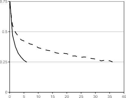

Figure 1: A four-layer convolutional neural network with ReLUs (solid line) reaches a 25% training error rate on CIFAR-10 six times faster than an equivalent network with tanh neurons (dashed line). The learning rates for each net- work were chosen independently to make train- ing as fast as possible. No regularization of any kind was employed. The magnitude of the effect demonstrated here varies with network architecture, but networks with ReLUs consis- tently learn several times faster than equivalents with saturating neurons.
Training on Multiple GPUs
单个 GTX 580 GPU 只有 3gb 内存,这限制了可以在其上训练的网络的最大大小。事实证明,120万个训练示例足以训练太大而无法安装在一个 GPU 上的网络。因此,我们将网络分布在两个 gpu 上。目前的 GPU 特别适合跨 GPU 并行化,因为它们可以直接从彼此的内存中读写,而无需通过主机内存。我们使用的并行化方案实际上将一半的内核 (或神经元) 放在每个 GPU 上,还有一个技巧: GPU 只在特定的层中通信。这意味着,例如,第三层的内核从第二层的所有内核映射中获取输入。然而,第四层的内核只从位于同一 GPU 上的第三层的内核映射中获取输入。选择连接模式是交叉验证的一个问题,但是这允许我们精确地调整通信量,直到它是计算量的可接受部分。
由此产生的体系结构与 Cires¸an 等人 [5] 使用的 “列” CNN 有些相似,只是我们的列不是独立的 (见图 2)。与在一个 GPU 上训练的每个卷积层内核数量为一半的网络相比,该方案分别降低了 1.7% 和 1.2% 的前 1 和前 5 错误率。与单 GPU net2 相比,双 GPU 网络的训练时间略少。
2 单 GPU 网络实际上与最终卷积层中的双 GPU 网络具有相同数量的内核。这是因为网络的大部分参数都在第一个全连接层中,该层将最后一个卷积层作为输入。因此,为了使两个网络具有大致相同的参数数量,我们没有将最终卷积层 (也没有将随后的完全连接层) 的大小减半。因此,这种比较偏向于单 GPU 网络,因为它比双 GPU 网络的 “一半大小” 大。
Local Response Normalization
略
Overlapping Pooling
Pooling layers in CNNs summarize the outputs of neighboring groups of neurons in the same kernel map. Traditionally, the neighborhoods summarized by adjacent pooling units do not overlap (e.g., [17, 11, 4]). To be more precise, a pooling layer can be thought of as consisting of a grid of pooling units spaced s _pixels apart, each summarizing a neighborhood of size _z z _centered at the location of the pooling unit. If we set _s = z, we obtain traditional local pooling as commonly employed in CNNs. If we set s < z, we obtain overlapping pooling. This is what we use throughout our network, with s = 2 and z = 3. This scheme reduces the top-1 and top-5 error rates by 0.4% and 0.3%, respectively, as compared with the non-overlapping scheme s = 2, z = 2, which produces output of equivalent dimensions. We generally observe during training that models with overlapping pooling find it slightly more difficult to overfit.
Overall Architecture
现在,我们准备描述 CNN 的整体架构。如图 2 所示,网络包含有权重的 8 层; 前 5 层是卷积的,其余 3 层是全连接的。最后一个全连接层的输出被送入 1000 路 softmax,该 softmax 在 1000 个类标签上产生分布。我们的网络最大化多项逻辑回归目标,这相当于在预测分布下最大化正确标签的对数概率的整个训练案例的平均值。
第二个、第四个和第五个卷积层的内核仅连接到位于同一 GPU 上的前一层中的内核映射 (见图 2)。第三卷积层的内核连接到第二层的所有内核映射。全连接层中的神经元与前一层中的所有神经元相连。响应标准化层遵循第一和第二个卷积层。第 3.4 节中描述的最大池化层遵循响应标准化层和第五个卷积层。将 ReLU 非线性应用于每个卷积和全连接层的输出。
The first convolutional layer filters the 224 224 3 input image with 96 kernels of size 11 11 3
with a stride of 4 pixels (this is the distance between the receptive field centers of neighboring
3We cannot describe this network in detail due to space constraints, but it is specified precisely by the code and parameter files provided here: http://code.google.com/p/cuda-convnet/.
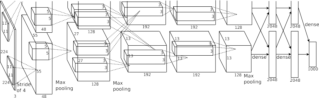
图 2: CNN 架构的一个例子,明确显示了两个 gpu 之间的职责划分。一个 GPU 运行图形顶部的图层部分,另一个 GPU 运行底部的图层部分。Gpu 只在某些层进行通信。网络的输入为 150,528 维,网络剩余层的神经元数量由 253,440-186,624-64,896-43,264-4096-1000 给出。
neurons in a kernel map). The second convolutional layer takes as input the (response-normalized and pooled) output of the first convolutional layer and filters it with 256 kernels of size 5 5 48. The third, fourth, and fifth convolutional layers are connected to one another without any intervening pooling or normalization layers. The third convolutional layer has 384 kernels of size 3 3 256 connected to the (normalized, pooled) outputs of the second convolutional layer. The fourth convolutional layer has 384 kernels of size 3 × _3 × 192 , and the fifth convolutional layer has 256 kernels of size 3 × 3 × _192. The fully-connected layers have 4096 neurons each.
Reducing Overfitting
我们的神经网络结构有 6000万个参数。尽管 ILSVRC 的 1000 个类使每个训练示例对从图像到标签的映射施加了 10 位约束,但事实证明,这不足以在没有大量过度拟合的情况下学习下面,我们描述了我们打击过度适应的两种主要方式。
数据增强
减少图像数据过度拟合的最简单和最常见的方法是使用保留标签的变换 (例如,[25,4,5) 人为放大数据集。我们采用了两种不同的数据增强形式,这两种形式都允许用很少的计算从原始图像中产生变换后的图像,因此变换后的图像不需要存储在在我们的实现中,当 GPU 对前一批图像进行训练时,转换后的图像是在 CPU 上的 Python 代码中生成的。因此,实际上,这些数据增强方案在计算上是免费的。
数据增强的第一种形式包括生成图像翻译和水平反射。我们通过随机抽取 224 224 补丁 (及其横向思考),
256 256 图像,并在这些提取的 patches4 上训练我们的网络。这将我们的培训规模增加了一个因素,即 2048年,尽管由此产生的培训例子当然是高度相互依存的。如果没有这个方案,我们的网络就会受到严重的过度拟合,这将迫使我们使用更小的网络。在测试时,网络通过提取五个 224 224 的补丁 (四个角补丁和中心补丁) 以及它们的水平反射 (因此总共有十个补丁) 来进行预测, 并对网络的 softmax 层在十个补丁上所做的预测进行平均。
数据增强的第二种形式是改变训练图像中 RGB 通道的强度。具体来说,我们在整个 ImageNet 训练集中对 RGB 像素值集执行 PCA。在每个训练图像中,我们添加找到的主成分的倍数,
4This is the reason why the input images in Figure 2 are 224 × _224 × _3-dimensional.
with magnitudes proportional to the corresponding eigenvalues times a random variable drawn from a Gaussian with mean zero and standard deviation 0.1. Therefore to each RGB image pixel I =
[IR , IG , IB ]_T _we add the following quantity:
xy xy xy
[p1, p2, p3][α_1λ1, α2λ2, α3λ3]_T
where p _and λ are _i_th eigenvector and eigenvalue of the 3 3 covariance matrix of RGB pixel values, respectively, and α is the aforementioned random variable. Each α _is drawn only once for all the pixels of a particular training image until that image is used for training again, at which point it is re-drawn. This scheme approximately captures an important property of natural images, namely, that object identity is invariant to changes in the intensity and color of the illumination. This scheme reduces the top-1 error rate by over 1%.
Dropout
Combining the predictions of many different models is a very successful way to reduce test errors [1, 3], but it appears to be too expensive for big neural networks that already take several days to train. There is, however, a very efficient version of model combination that only costs about a factor of two during training. The recently-introduced technique, called “dropout” [10], consists of setting to zero the output of each hidden neuron with probability 0.5. The neurons which are “dropped out” in this way do not contribute to the forward pass and do not participate in back- propagation. So every time an input is presented, the neural network samples a different architecture, but all these architectures share weights. This technique reduces complex co-adaptations of neurons, since a neuron cannot rely on the presence of particular other neurons. It is, therefore, forced to learn more robust features that are useful in conjunction with many different random subsets of the other neurons. At test time, we use all the neurons but multiply their outputs by 0.5, which is a reasonable approximation to taking the geometric mean of the predictive distributions produced by the exponentially-many dropout networks.
We use dropout in the first two fully-connected layers of Figure 2. Without dropout, our network ex- hibits substantial overfitting. Dropout roughly doubles the number of iterations required to converge.
Details of learning
 We trained our models using stochastic gradient descent with a batch size of 128 examples, momentum of 0.9, and weight decay of 0.0005. We found that this small amount of weight decay was important for the model to learn. In other words, weight decay here is not merely a regularizer: it reduces the model’s training error. The update rule for weight _w _was
Results
Our results on ILSVRC-2010 are summarized in Table 1. Our network achieves top-1 and top-5 test set error rates of 37.5% and 17.0%5. The best performance achieved during the ILSVRC- 2010 competition was 47.1% and 28.2% with an approach that averages the predictions produced from six sparse-coding models trained on different features [2], and since then the best pub- lished results are 45.7% and 25.7% with an approach that averages the predictions of two classi- fiers trained on Fisher Vectors (FVs) computed from two types of densely-sampled features [24].
We also entered our model in the ILSVRC-2012 com- petition and report our results in Table 2. Since the ILSVRC-2012 test set labels are not publicly available, we cannot report test error rates for all the models that we tried. In the remainder of this paragraph, we use
| Model | Top-1 | Top-5 |
|---|---|---|
| Sparse coding [2] | 47.1% | 28.2% |
| SIFT + FVs [24] | 45.7% | 25.7% |
| CNN | 37.5% | 17.0% |
validation and test error rates interchangeably because in our experience they do not differ by more than 0.1% (see Table 2). The CNN described in this paper achieves a top-5 error rate of 18.2%. Averaging the predictions
Table 1: Comparison of results on ILSVRC-
2010 test set. In _italics _are best results achieved by others.
of five similar CNNs gives an error rate of 16.4%. Training one CNN, with an extra sixth con- volutional layer over the last pooling layer, to classify the entire ImageNet Fall 2011 release (15M images, 22K categories), and then “fine-tuning” it on ILSVRC-2012 gives an error rate of 16.6%. Averaging the predictions of two CNNs that were pre-trained on the entire Fall 2011 re- lease with the aforementioned five CNNs gives an error rate of 15.3%. The second-best con- test entry achieved an error rate of 26.2% with an approach that averages the predictions of sev- eral classifiers trained on FVs computed from different types of densely-sampled features [7].
Finally, we also report our error rates on the Fall 2009 version of ImageNet with 10,184 categories and 8.9 million images. On this dataset we follow the convention in the literature of using half of the images for training and half for testing. Since there is no es-
| Model | Top-1 (val) | Top-5 (val) | Top-5 (test) |
|---|---|---|---|
| SIFT + FVs [7] | — | — | 26.2% |
| 1 CNN | 40.7% | 18.2% | — |
| 5 CNNs | 38.1% | 16.4% | 16.4% |
| 1 CNN* | 39.0% | 16.6% | — |
| 7 CNNs* | 36.7% | 15.4% | 15.3% |
tablished test set, our split neces- sarily differs from the splits used by previous authors, but this does not affect the results appreciably. Our top-1 and top-5 error rates on this dataset are 67.4% and
Table 2: Comparison of error rates on ILSVRC-2012 validation and test sets. In _italics _are best results achieved by others. Models with an asterisk* were “pre-trained” to classify the entire ImageNet 2011 Fall release. See Section 6 for details.
40.9%, attained by the net described above but with an additional, sixth convolutional layer over the last pooling layer. The best published results on this dataset are 78.1% and 60.9% [19].
6.1 Qualitative Evaluations
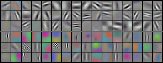
Figure 3 shows the convolutional kernels learned by the network’s two data-connected layers. The network has learned a variety of frequency- and orientation-selective kernels, as well as various col- ored blobs. Notice the specialization exhibited by the two GPUs, a result of the restricted connec- tivity described in Section 3.5. The kernels on GPU 1 are largely color-agnostic, while the kernels on on GPU 2 are largely color-specific. This kind of specialization occurs during every run and is independent of any particular random weight initialization (modulo a renumbering of the GPUs).
5The error rates without averaging predictions over ten patches as described in Section 4.1 are 39.0% and 18.3%.
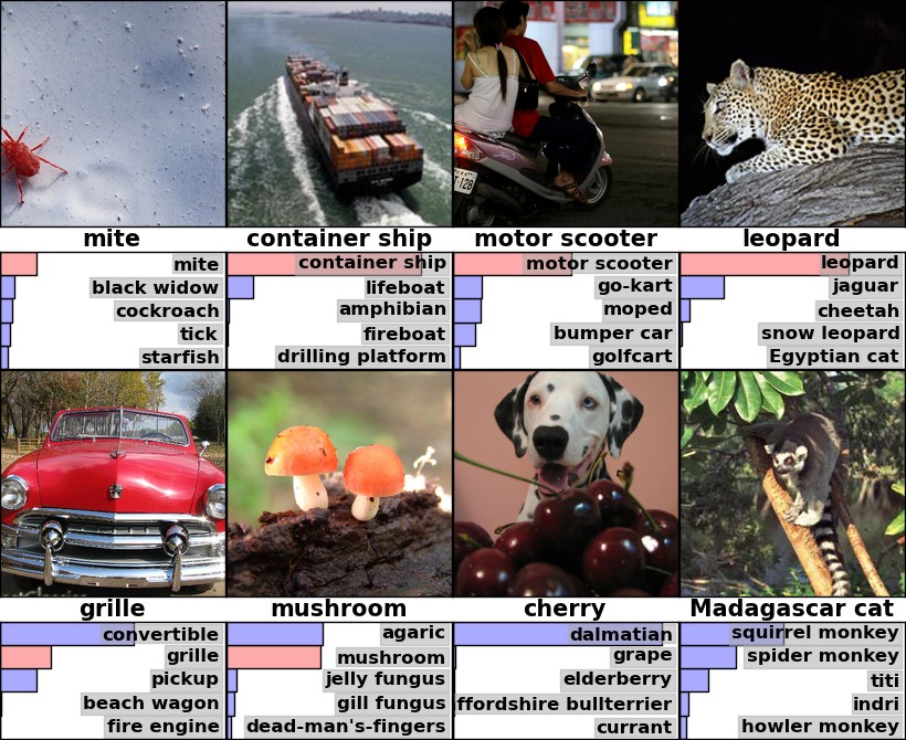
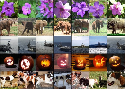
Figure 4: (Left) Eight ILSVRC-2010 test images and the five labels considered most probable by our model. The correct label is written under each image, and the probability assigned to the correct label is also shown with a red bar (if it happens to be in the top 5). (Right) Five ILSVRC-2010 test images in the first column. The remaining columns show the six training images that produce feature vectors in the last hidden layer with the smallest Euclidean distance from the feature vector for the test image.
In the left panel of Figure 4 we qualitatively assess what the network has learned by computing its top-5 predictions on eight test images. Notice that even off-center objects, such as the mite in the top-left, can be recognized by the net. Most of the top-5 labels appear reasonable. For example, only other types of cat are considered plausible labels for the leopard. In some cases (grille, cherry) there is genuine ambiguity about the intended focus of the photograph.
Another way to probe the network’s visual knowledge is to consider the feature activations induced by an image at the last, 4096-dimensional hidden layer. If two images produce feature activation vectors with a small Euclidean separation, we can say that the higher levels of the neural network consider them to be similar. Figure 4 shows five images from the test set and the six images from the training set that are most similar to each of them according to this measure. Notice that at the pixel level, the retrieved training images are generally not close in L2 to the query images in the first column. For example, the retrieved dogs and elephants appear in a variety of poses. We present the results for many more test images in the supplementary material.
Computing similarity by using Euclidean distance between two 4096-dimensional, real-valued vec- tors is inefficient, but it could be made efficient by training an auto-encoder to compress these vectors to short binary codes. This should produce a much better image retrieval method than applying auto- encoders to the raw pixels [14], which does not make use of image labels and hence has a tendency to retrieve images with similar patterns of edges, whether or not they are semantically similar.
Discussion
Our results show that a large, deep convolutional neural network is capable of achieving record- breaking results on a highly challenging dataset using purely supervised learning. It is notable that our network’s performance degrades if a single convolutional layer is removed. For example, removing any of the middle layers results in a loss of about 2% for the top-1 performance of the network. So the depth really is important for achieving our results.
To simplify our experiments, we did not use any unsupervised pre-training even though we expect that it will help, especially if we obtain enough computational power to significantly increase the size of the network without obtaining a corresponding increase in the amount of labeled data. Thus far, our results have improved as we have made our network larger and trained it longer but we still have many orders of magnitude to go in order to match the infero-temporal pathway of the human visual system. Ultimately we would like to use very large and deep convolutional nets on video sequences where the temporal structure provides very helpful information that is missing or far less obvious in static images.
References
[1]R.M. Bell and Y. Koren. Lessons from the netflix prize challenge. ACM SIGKDD Explorations Newsletter, 9(2):75–79, 2007.
[2]A. Berg, J. Deng, and L. Fei-Fei. Large scale visual recognition challenge 2010. www.image- net.org/challenges. 2010.
[3]L. Breiman. Random forests. Machine learning, 45(1):5–32, 2001.
[4]D. Cires¸an, U. Meier, and J. Schmidhuber. Multi-column deep neural networks for image classification.
Arxiv preprint arXiv:1202.2745, 2012.
[5]D.C. Cires¸an, U. Meier, J. Masci, L.M. Gambardella, and J. Schmidhuber. High-performance neural networks for visual object classification. Arxiv preprint arXiv:1102.0183, 2011.
[6]J. Deng, W. Dong, R. Socher, L.-J. Li, K. Li, and L. Fei-Fei. ImageNet: A Large-Scale Hierarchical Image Database. In CVPR09, 2009.
[7]J. Deng, A. Berg, S. Satheesh, H. Su, A. Khosla, and L. Fei-Fei. ILSVRC-2012, 2012. URL
http://www.image-net.org/challenges/LSVRC/2012/.
[8]L. Fei-Fei, R. Fergus, and P. Perona. Learning generative visual models from few training examples: An incremental bayesian approach tested on 101 object categories. Computer Vision and Image Understand- ing, 106(1):59–70, 2007.
[9]G. Griffin, A. Holub, and P. Perona. Caltech-256 object category dataset. Technical Report 7694, Cali- fornia Institute of Technology, 2007. URL http://authors.library.caltech.edu/7694.
[10]G.E. Hinton, N. Srivastava, A. Krizhevsky, I. Sutskever, and R.R. Salakhutdinov. Improving neural net- works by preventing co-adaptation of feature detectors. arXiv preprint arXiv:1207.0580, 2012.
[11]K. Jarrett, K. Kavukcuoglu, M. A. Ranzato, and Y. LeCun. What is the best multi-stage architecture for object recognition? In International Conference on Computer Vision, pages 2146–2153. IEEE, 2009.
[12]A. Krizhevsky. Learning multiple layers of features from tiny images. Master’s thesis, Department of Computer Science, University of Toronto, 2009.
[13]A. Krizhevsky. Convolutional deep belief networks on cifar-10. Unpublished manuscript, 2010.
[14]A. Krizhevsky and G.E. Hinton. Using very deep autoencoders for content-based image retrieval. In
ESANN, 2011.
[15]Y. Le Cun, B. Boser, J.S. Denker, D. Henderson, R.E. Howard, W. Hubbard, L.D. Jackel, et al. Hand- written digit recognition with a back-propagation network. In Advances in neural information processing systems, 1990.
[16]Y. LeCun, F.J. Huang, and L. Bottou. Learning methods for generic object recognition with invariance to pose and lighting. In Computer Vision and Pattern Recognition, 2004. CVPR 2004. Proceedings of the 2004 IEEE Computer Society Conference on, volume 2, pages II–97. IEEE, 2004.
[17]Y. LeCun, K. Kavukcuoglu, and C. Farabet. Convolutional networks and applications in vision. In Circuits and Systems (ISCAS), Proceedings of 2010 IEEE International Symposium on, pages 253–256. IEEE, 2010.
[18]H. Lee, R. Grosse, R. Ranganath, and A.Y. Ng. Convolutional deep belief networks for scalable unsuper- vised learning of hierarchical representations. In Proceedings of the 26th Annual International Conference on Machine Learning, pages 609–616. ACM, 2009.
[19]T. Mensink, J. Verbeek, F. Perronnin, and G. Csurka. Metric Learning for Large Scale Image Classifi- cation: Generalizing to New Classes at Near-Zero Cost. In ECCV - European Conference on Computer Vision, Florence, Italy, October 2012.
[20]V. Nair and G. E. Hinton. Rectified linear units improve restricted boltzmann machines. In Proc. 27th International Conference on Machine Learning, 2010.
[21]N. Pinto, D.D. Cox, and J.J. DiCarlo. Why is real-world visual object recognition hard? PLoS computa- tional biology, 4(1):e27, 2008.
[22]N. Pinto, D. Doukhan, J.J. DiCarlo, and D.D. Cox. A high-throughput screening approach to discovering good forms of biologically inspired visual representation. PLoS computational biology, 5(11):e1000579, 2009.
[23]B.C. Russell, A. Torralba, K.P. Murphy, and W.T. Freeman. Labelme: a database and web-based tool for image annotation. International journal of computer vision, 77(1):157–173, 2008.
[24]J. Sánchez and F. Perronnin. High-dimensional signature compression for large-scale image classification. In Computer Vision and Pattern Recognition (CVPR), 2011 IEEE Conference on, pages 1665–1672. IEEE, 2011.
[25]P.Y. Simard, D. Steinkraus, and J.C. Platt. Best practices for convolutional neural networks applied to visual document analysis. In Proceedings of the Seventh International Conference on Document Analysis and Recognition, volume 2, pages 958–962, 2003.
[26]S.C. Turaga, J.F. Murray, V. Jain, F. Roth, M. Helmstaedter, K. Briggman, W. Denk, and H.S. Seung. Con- volutional networks can learn to generate affinity graphs for image segmentation. Neural Computation, 22(2):511–538, 2010.

若有收获,就点个赞吧
0 人点赞
