- 让我们导入Fashion-MNIST数据集
- 测量我们模型的准确性
- 训练我们的模型
- 为了清楚的说明
- 过度拟合
- 正则
- 推理
- 结论
- repository for the full code!">Thank you so much for your time, and please check out this repository for the full code!
medium
有人可能会争辩说,最好是过拟合你的模型,然后对其进行逆向工程而不是相反。
在这个项目中,我们可以看到将Dropout正则化实现到神经网络后的准确性和验证损失的差异。 我们将使用PyTorch库从头开始构建一个顺序神经网络,以便在fashion-MNIST数据集中对10个不同的类进行分类。 这个数据集是28x28灰度图像的衣服。 我们将深入研究dropout的方法,并证明它是否能防止过度拟合。
该项目的灵感来自:
Facebook Udacity PyTorch Challenge.
首先,我们将创建一个没有正则化实现的神经网络,我们的假设是我们可以推断,随着时间的推移,我们的模型在验证集中表现不佳,因为我们用训练集训练我们的模型越多, 通过对测试数据的特定特征进行分类则越好,从而创建不良的泛化模型去推理。
让我们导入Fashion-MNIST数据集
让我们使用torchvision下载数据集,通常我们将20%的数据集分开用于验证集。 但在这种情况下,我们将直接从torchvision下载数据集。
import torchfrom torchvision import datasets, transformsimport helpertransform = transforms.Compose([transforms.ToTensor(),transforms.Normalize((0.5,0.5,0.5),(0.5,0.5,0.5))])traindataset = datasets.FashionMNIST('~/.pytorch/F_MNIST_data/', download=True,train=True,transform=transform)trainloader = torch.utils.data.DataLoader(dataset=traindataset, batch_size=64, shuffle=True)testdataset = datasets.FashionMNIST('~/.pytorch/F_MNIST_data/', download=True,train=False,transform=transform)testloader = torch.utils.data.DataLoader(dataset=testdataset, batch_size=64, shuffle=True)
我们需要导入torchvision来下载数据集和转换。 然后我们使用变换库将图像转换为张量并进行标准化。 通常批量训练和验证集以提高训练速度并且改组数据也会增加训练和测试数据的学习差异。
定义神经网络
这个模型将有2个隐藏层,输入层将有784个单元,并且在最终层将有10个输出,因为我们有10个不同的类进行分类。 我们将使用交叉熵损失,因为它具有对数性质,可以将我们的输出归一化到接近零或一。
from torch import nnfrom torch.functional import Fclass FashionNeuralNetwork(nn.Module):def __init__(self):super().__init__()# Create layers hereself.layer_input = nn.Linear(784,256)self.layer_hidden_one = nn.Linear(256,128)self.layer_hidden_two = nn.Linear(128,64)self.layer_output = nn.Linear(64,10)def forward(self, x):# Flattened the input to make sure it fits the layer inputx = x.view(x.shape[0],-1)# Pass in the input to the layer and do forward propagationx = F.relu(self.layer_input(x))x = F.relu(self.layer_hidden_one(x))x = F.relu(self.layer_hidden_two(x))# Dimension = 1x = F.log_softmax(self.layer_output(x),dim=1)return x
该神经网络将使用ReLU作为隐藏层的非线性激活函数,并使用log-softmax激活输出和负对数似然函数用于我们的损失函数。 如果我们查看PyTorch库中的交叉熵损失的文档,该标准将nn.LogSoftmax()和nn.NLLLoss()组合在一个单独的类中。 损失可以描述为: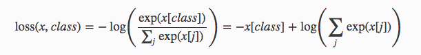
请注意,转发传播结束时的线性函数的dim = 1,这意味着输出结果的每一行的概率总和必须等于1.给单个元素的概率最高图像的概率最高 被归类为相应的类索引。
我们必须确保模型的输出形状正确性,
# Instantiate the modelmodel = FashionNeuralNetwork()# Get the images and labels from the test loaderimages, labels = next(iter(testloader))# Get the log probability prediction from our modellog_ps = model(images)# Normalize the probability by taking the exponent of the log-probps = torch.exp(log_ps)# Print out the sizeprint(ps.shape)
确保输出为:
torch.Size([64, 10])
测量我们模型的准确性
由于我们想要一个类的最高概率,我们将使用ps.topk来获得top-k值和top-k索引的元组,例如,如果在4个元素中最高为kth,我们将得到3作为指数。
top_p, top_class = ps.topk(1,dim=1)# Print out the most likely classes for the first 10 examplesprint(top_class[:10,:])
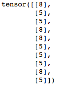
top_class是尺寸为64x1的2D张量,而我们的标签是尺寸为64的1D张量。为了测量标签和模型预测之间的准确度,我们必须确保张量的形状是相同的。
# We have to reshape the labels to 64x1 using the view() methodequals = top_class == labels.view(*top_class.shape)print(equals.shape)
比较张量的输出将是:
torch.Size([64, 1])
为了计算模型的准确性,我们只需计算模型正确预测的次数。 如果我们的预测与标签相同,则上面的==运算符将逐行检查。 最终结果将是二进制0不相同,1正确预测。 我们可以使用torch.mean计算平均值,但我们需要将equals转换为FloatTensor。
accuracy = torch.mean(equals.type(torch.FloatTensor))# Print the accuracyprint(f'Accuracy: {accuracy.item()*100}%')
训练我们的模型
由于我们希望损失函数与Logarithm Softmax函数的行为相反,我们将使用负对数似然来计算我们的损失。
from torch import optim# Instantiate the modelmodel = FashionNeuralNetwork()# Use Negative Log Likelyhood as our loss functionloss_function = nn.NLLLoss()# Use ADAM optimizer to utilize momentumoptimizer = optim.Adam(model.parameters(), lr=0.003)# Train the model 30 cyclesepochs = 30# Initialize two empty arrays to hold the train and test lossestrain_losses, test_losses = [],[]# Start the trainingfor i in range(epochs):running_loss = 0# Loop through all of the train set forward and back propagatefor images,labels in trainloader:optimizer.zero_grad()log_ps = model(images)loss = loss_function(log_ps, labels)loss.backward() # Backpropagateoptimizer.step()running_loss += loss.item()# Initialize test loss and accuracy to be 0test_loss = 0accuracy = 0# Turn off the gradientswith torch.no_grad():# Loop through all of the validation setfor images, labels in testloader:log_ps = model(images)ps = torch.exp(log_ps)test_loss += loss_function(log_ps, labels)top_p, top_class = ps.topk(1,dim=1)equals = top_class == labels.view(*top_class.shape)accuracy += torch.mean(equals.type(torch.FloatTensor))# Append the average losses to the array for plottingtrain_losses.append(running_loss/len(trainloader))test_losses.append(test_loss/len(testloader))
打印我们的模型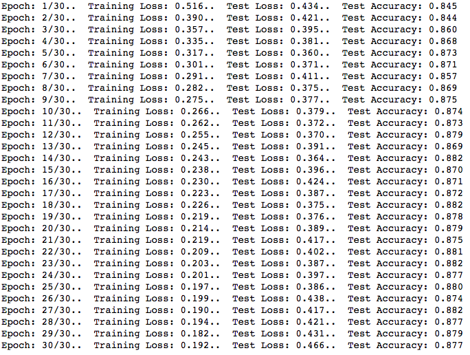
这证明了我们的假设,即完全说明我们的模型将训练的很好,但不能推广训练数据集之外的图像。 我们可以看到,30个周期的训练损失显著减少,但我们的验证损失在大约36-48%之间波动。 这是过度拟合的标志,这个情况说明,模型学习训练数据集的特定特征和模式,它无法正确分类数据集之外的图像。 这通常很糟糕,因为这意味着如果我们使用推理,模型就无法正确分类。
为了清楚的说明
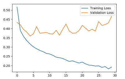
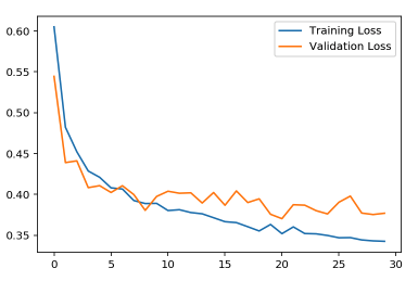
让我们画图看一下:
# Plot the graph here%matplotlib inline%config InlineBackend.figure_format = 'retina'import matplotlib.pyplot as pltplt.plot(train_losses, label='Training Loss')plt.plot(test_losses, label='Validation Loss')plt.legend(frameon=True)
过度拟合
从上图中我们可以清楚地看到,我们的模型并没有很好地泛华。 这意味着该模型在对训练数据集之外的图像进行分类方面做得不好。 这真的很糟糕,这意味着我们的模型只学习我们的训练数据集的具体内容,它变得如此个别,以至于它只能识别来自训练集的图像。 如果我们从图表中看到,每个周期的训练损失都会显著减少,但是,我们可以看到验证损失却没发生什么变化。
正则
这就是正则化的用武之地,其中一种方法是进行L2正则化,也称为early-stopping,这基本上意味着我们将在验证损失最低时停止训练我们的模型。 在这种情况下,我们的验证损失在3-5个时期后达到最佳。 这意味着超过5个周期,我们的模型泛化会变得更糟。
但是,还有另一种方法可以解决这个问题。 我们可以为我们的模型进行dropout,以进行更多的泛化。 基本上,我们的模型通过在大型重量上滚雪球并使其他要训练的重量不足而贪婪地行动。 通过具有随机丢失,具有较小权重的节点将有机会在循环期间被训练,从而在结束时给出更一般化的分数。 换句话说,它迫使网络在权重之间共享信息,从而提供更好的泛化能力。
注意:
在训练期间,我们希望实行dropout,但是,在验证过程中,我们需要我们模型的全部功能,因为那时我们可以完全测量模型对这些图像进行泛化其准确性。 如果我们使用model.eval()模式,我们将停止使用dropout,并且不要忘记在训练期间使用model.train()再次使用它。
### Define our new Network with Dropoutsclass FashionNeuralNetworkDropout(nn.Module):def __init__(self):super().__init__()# Create layers hereself.layer_input = nn.Linear(784,256)self.layer_hidden_one = nn.Linear(256,128)self.layer_hidden_two = nn.Linear(128,64)self.layer_output = nn.Linear(64,10)# 20% Dropout hereself.dropout = nn.Dropout(p=0.2)def forward(self, x):# Flattened the input to make sure it fits the layer inputx = x.view(x.shape[0],-1)# Pass in the input to the layer and do forward propagationx = self.dropout(F.relu(self.layer_input(x)))x = self.dropout(F.relu(self.layer_hidden_one(x)))x = self.dropout(F.relu(self.layer_hidden_two(x)))# Dimension = 1x = F.log_softmax(self.layer_output(x),dim=1)return x
这个神经网络将与第一个模型非常相似,但是,我们将增加20%的丢失。 现在让我们训练这个模型吧!
from torch import optim# Instantiate the modelmodel = FashionNeuralNetworkDropout()# Use Negative Log Likelyhood as our loss functionloss_function = nn.NLLLoss()# Use ADAM optimizer to utilize momentumoptimizer = optim.Adam(model.parameters(), lr=0.003)# Train the model 30 cyclesepochs = 30# Initialize two empty arrays to hold the train and test lossestrain_losses, test_losses = [],[]# Start the trainingfor i in range(epochs):running_loss = 0# Loop through all of the train set forward and back propagatefor images,labels in trainloader:optimizer.zero_grad()log_ps = model(images)loss = loss_function(log_ps, labels)loss.backward() # Backpropagateoptimizer.step()running_loss += loss.item()# Initialize test loss and accuracy to be 0test_loss = 0accuracy = 0# Turn off the gradientswith torch.no_grad():# Turn on Evaluation modemodel.eval()# Loop through all of the validation setfor images, labels in testloader:log_ps = model(images)ps = torch.exp(log_ps)test_loss += loss_function(log_ps, labels)top_p, top_class = ps.topk(1,dim=1)equals = top_class == labels.view(*top_class.shape)accuracy += torch.mean(equals.type(torch.FloatTensor))# Turn on Training mode againmodel.train()# Append the average losses to the array for plottingtrain_losses.append(running_loss/len(trainloader))test_losses.append(test_loss/len(testloader))
输出结果: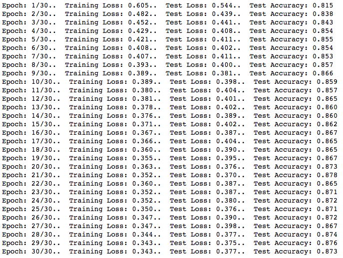
这里的目标是使验证损失与我们的训练损失一样低,这意味着我们的模型相当准确。 让我们再次绘制图表,看看正则化后的差异。 即使精度水平仅整体上升0.3%,该模型也没有过度拟合,因为它保持了在训练期间训练的所有节点的平衡。 让我们绘制图表并查看差异:
# Plot the graph here%matplotlib inline%config InlineBackend.figure_format = 'retina'import matplotlib.pyplot as pltplt.plot(train_losses, label='Training Loss')plt.plot(test_losses, label='Validation Loss')plt.legend(frameon=True)
推理
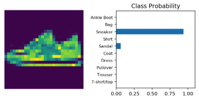
现在我们的模型可以更好地泛化,让我们用提供模型尝试用训练数据集之外的图像进行预测,并可视化模型的分类。
# Make sure to make our model in the evaluation modemodel.eval()# Get the next image and labelimages, labels = next(iter(testloader))img = images[0]# Convert 2D image to 1D vectorimg = img.view(1, 784)# Calculate the class probabilities (log-softmax) for imgwith torch.no_grad():output = model.forward(img)# Normalize the outputps = torch.exp(output)# Plot the image and probabilitieshelper.view_classify(img.view(1, 28, 28), ps, version='Fashion')
结论
这很棒! 我们可以看到培训损失和验证损失之间的显着平衡。 可以肯定地说,如果我们训练模型进行更多循环并微调我们的超参数,则验证损失将减少。 从上图中我们可以看出,我们的模型随着时间的推移更好地泛化,模型在6-8个时期之后可以获得更好的精度,并且可以肯定地说模型通过实现模型的丢失来防止过度拟合。
Thank you so much for your time, and please check out this repository for the full code!

若有收获,就点个赞吧
0 人点赞
