Snips Voice Platform: an embedded
Spoken Language Understanding system for private-by-design voice interfaces
| Alice Coucke | Alaa Saade | Adrien Ball |
|---|---|---|
| Théodore Bluche | Alexandre Caulier | David Leroy |
| Clément Doumouro | Thibault Gisselbrecht | Francesco Caltagirone |
| Thibaut Lavril | Maël Primet Snips Paris, France Abstract |
Joseph Dureau |
This paper presents the machine learning architecture of the Snips Voice Platform, a software solution to perform Spoken Language Understanding on microprocessors typical of IoT devices. The embedded inference is fast and accurate while enforcing privacy by design, as no personal user data is ever collected. Focusing on Automatic Speech Recognition and Natural Language Understanding, we detail our approach to training high-performance Machine Learning models that are small enough to run in real-time on small devices. Additionally, we describe a data generation procedure that provides sufficient, high-quality training data without compromising user privacy.
1 Introduction
Over the last years, thanks in part to steady improvements brought by deep learning approaches to speech recognition [33, 17, 14, 5], voice interfaces have greatly evolved from spotting limited and predetermined keywords to understanding arbitrary formulations of a given intention. They also became much more reliable, with state-of-the-art speech recognition engines reaching human level in English [56]. This achievement unlocked many practical applications of voice assistants which are now used in many fields from customer support [6, 47], to autonomous cars [41], or smart homes [16, 26]. In particular, smart speaker adoption by the public is on the rise, with a recent study showing that nearly 20% of U.S. adults reported having a smart speaker at home[1].
These recent developments however raise questions about user privacy – especially since unique speaker identification is an active field of research using voice as a sensitive biometric feature [58]. The CNIL (French Data Protection Authority)[2]advises owners of connected speakers to switch off the microphone when possible and to warn guests of the presence of such a device in their home. The General Data Protection Regulation which harmonizes data privacy laws across the European Union[3]indeed requires companies to ask for explicit consent before collecting user data.
Some of the most popular commercial solutions for voice assistants include Microsoft’s Cortana, Google’s DialogFlow, IBM’s Watson, or Amazon Alexa [23]. In this paper, we introduce a competing solution, the Snips Voice Platform which, unlike the previous ones, is completely cloud independent and runs offline on typical IoT microprocessors, thus guaranteeing privacy by design, with no user data ever collected nor stored. The Natural Language Understanding component of the platform is already open source [50], while the other components will be opensourced in the future.
The aim of this paper is to contribute to the collective effort towards ever more private and efficient cloud-independent voice interfaces. To this end, we devote this introduction to a brief description of the Snips Ecosystem and of some of the design principles behind the Snips Voice Platform.
1.1 The Snips Ecosystem
The Snips ecosystem comprises a web console[4]to build voice assistants and train the corresponding Spoken Language Understanding (SLU) engine, made of an Automatic Speech Recognition (ASR) engine and a Natural Language Understanding (NLU) engine. The console can be used as a selfservice development environment by businesses or individuals, or through professional services. The Snips Voice Platform is free for non-commercial use. Since its launch in Summer 2017, over 23,000 Snips voice assistants have been created by over 13,000 developers. The languages currently supported by the Snips platform are English, French and German, with additional NLU support for Spanish and Korean. More languages are added regularly.
An assistant _is composed of a set of _skills – e.g. SmartLights, SmartThermostat, or SmartOven skills for a SmartHome assistant – that may be either selected from preexisting ones in a skill store _or created from scratch on the web console. A given skill may contain several _intents, or user intention – e.g. SwitchLightOn and SwitchLightOff for a SmartLights skill. Finally, a given intent is bound to a list of entities _that must be extracted from the user’s query – e.g. room for the SwitchLightOn intent. We call _slot _the particular value of an entity in a query – e.g. kitchen for the entity room. When a user speaks to the assistant, the SLU engine trained on the different skills will handle the request by successively converting speech into text, classifying the user’s intent, and extracting the relevant slots.
Once the user’s request has been processed and based on the information that has been extracted from the query and fed to the device, a dialog management component is responsible for providing a feedback to the user, or performing an _action. It may take multiple forms, such as an audio response via speech synthesis or a direct action on a connected device – e.g. actually turning on the lights for a SmartLights skill. Figure 1 illustrates the typical interaction flow.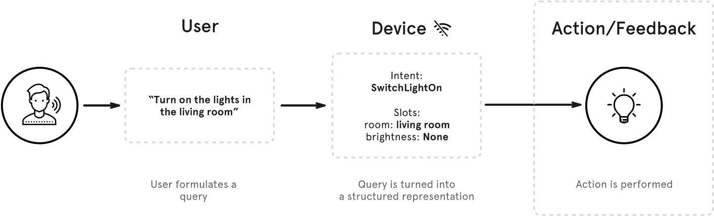
Figure 1: Interaction flow
1.2 A private-by-design embedded platform
The Privacy by Design [10, 25] principle sets privacy as the default standard in the design and engineering of a system. In the context of voice assistants, that can be deployed anywhere including users’ homes, this principle calls for a strong interpretation to protect users against any future misuse of their private data. In the following, we call _private-by-design _a system that does not transfer user data to any remote location, such as cloud servers.
Within the Snips ecosystem, the SLU components are trained on servers, but the inference happens directly on the device once the assistant has been deployed - no data from the user is ever collected nor stored. This design choice adds engineering complexity as most IoT devices run on specific hardware with limited memory and computing power. Cross-platform support is also a requirement in the IoT industry, since IoT devices are powered by many different hardware boards, with sustained innovation in that field.
For these reasons, the Snips Voice Platform has been built with portability and footprint in mind. Its embedded inference runs on common IoT hardware as light as the Raspberry Pi 3 (CPU with 1.4 GHz and 1GB of RAM), a popular choice among developers and therefore our reference hardware setting throughout this paper. Other Linux boards are also supported, such as IMX.7D, i.MX8M, DragonBoard 410c, and Jetson TX2. The Snips SDK for Android works with devices with Android 5 and ARM CPU, while the iOS SDK targets iOS 11 and newer. For efficiency and portability reasons, the algorithms have been re-implemented whenever needed in Rust [29] – a modern programming language offering high performance, low memory overhead, and cross-compilation.
SLU engines are usually broken down into two parts: Automatic Speech Recognition (ASR) and Natural Language Understanding (NLU). The ASR engine translates a spoken utterance into text through an acoustic model, mapping raw audio to a phonetic representation, and a Language Model (LM), mapping this phonetic representation to text. The NLU then extracts intent and slots from the decoded query. As discussed in section 3, LM and NLU have to be mutually consistent in order to optimize the accuracy of the SLU engine. It is therefore useful to introduce a _language modeling _component composed of the LM and NLU. Figure 2 describes the building blocks of the SLU pipeline.

Figure 2: Spoken Language Understanding pipeline
As stated above, ASR engines relying on large deep learning models have improved drastically over the past few years. Yet, they still have a major drawback today. For example, the model achieving human parity in [56] is a combination of several neural networks, each containing several hundreds of millions of parameters, and large-vocabulary language models made of several millions of n-grams. The size of these models, along with the computational resources necessary to run them in real-time, make them unfit for deployment on small devices, so that solutions implementing them are bound to rely on the cloud for speech recognition.
Enforcing privacy by design therefore implies developing new tools to build reliable SLU engines that are constrained in size and computational requirements, which we detail in this paper. In section 2, we describe strategies to obtain small (10MB) and robust acoustic models trained on general speech corpora of a few hundred to a few thousand hours. Section 3 is devoted to a description of the language modeling approach of the Snips SLU engine. Notably, we show how to ensure consistency between the language model of the ASR engine and the NLU engine while specializing them to a particular use case. The resulting SLU engine is lightweight and fast to execute, making it fit for deployment on small devices and the NLU component is open source [50]. In section 4, we illustrate the high generalization accuracy of the SLU engine in the context of real-word voice assistants. Finally, we discuss in section 9 a data generation procedure to automatically create training sets replacing user data.
2 Acoustic model
The acoustic model is the first step of the SLU pipeline, and is therefore crucial to its functioning. If the decoding contains errors, it might compromise the subsequent steps and trigger a different action than that intended by the user.
The acoustic model is responsible for converting raw audio data to what can approximately be interpreted as phone probabilities, i.e. context-dependent clustered Hidden Markov Model (HMM) state probabilities. These probabilities are then fed to a language model, which decodes a sequence of words corresponding to the user utterance. The acoustic and language models are thus closely related in the Automatic Speech Recognition (ASR) engine, but are often designed and trained separately. The construction of the language model used in the SLU engine is detailed in section 3.
In this section, we present the acoustic model. First, we give details about how the training data is collected, processed, cleaned, and augmented. Then, we present the acoustic model itself (a hybrid of Neural Networks and Hidden Markov Models, or NN/HMM) and how it is trained. Finally, we present the performance of the acoustic model in a large-vocabulary setup, in terms of word error rate (WER), speed, and memory usage.
2.1 Data
Training data. To train the acoustic model, we need several hundreds to thousands of hours of audio data with corresponding transcripts. The data is collected from public or commercial sources. A realignment of transcripts to the audio is performed to match transcripts to timestamps. This additionally helps in removing transcription errors that might be present in the data. The result is a set of audio extracts and matching transcripts, with lengths suitable for acoustic training (up to a few dozen seconds). This data is split in a training, testing, and development sets.
Data augmentation. One of the main issues regarding the training of the acoustic model is the lack of data corresponding to real usage scenari. Most of the available training data is clear close-field speech, but voice assistants will often be used in noisy conditions (music, television, environment noise), from a distance of several meters in far-field conditions, and in rooms or cars with reverberation. From a machine learning perspective, data corresponding to real usage of the system — or in-domain data – is extremely valuable. Since spoken utterances from the user are not collected by our platform for privacy reasons, noisy and reverberant conditions are simulated by augmenting the data. Thousands of virtual rooms of different sizes are thus generated with random microphone and speaker locations, and the rerecording of the original data in those conditions is simulated using a method close to that presented in [22].
2.2 Model training
Acoustic models are hybrid NN/HMM models. More specifically, they are a custom version of the s5 training recipe of the Kaldi toolkit [42]. 40 MFCC features are extracted from the audio signal with windows of size 25ms every 10ms.
Models with a variable number of layers and neurons can be trained, which will impact their accuracy and computational cost. We can thus train different model architectures depending on the target hardware and the desired application accuracy. In the following evaluation (section 2.3), we present performance results of a model targeted for the Raspberry Pi 3.
First, a speaker-adaptive Gaussian Mixture Model Hidden Markov Model (GMM-HMM) is trained on the speech corpus to obtain a context-dependent bootstrapping model with which we align the full dataset and extract lattices to prepare the neural network training.
We train a deep neural network, consisting of time-delay layers similar to those presented in [39], and long short-term memory layers similar to those of [40]. The architecture, close to that of [40], is summarized in Figure 3 and Table 1. The Raspberry Pi 3 model uses 7 layers, and is trained with the lattice-free Maximum Mutual Information (MMI) criterion [43], using natural gradient descent, with a learning rate of 0.0005 and the backstitching trick [55]. We follow the approach described in [43] to create fast acoustic models, namely an HMM topology with one state for each of the 1,700 context-dependent senones, operating at a third of the original frame rate.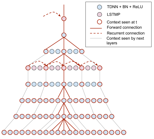
Figure 3: The TDNN-LSTM architecture used in the presented models.
Table 1: Network architecture. The _Context _denotes the number of relative frames seen by the layer at time t. For instance, the recurrent connections skip 3 frames in LSTMP layers. A projection layer size of _N _is denoted pN. (TDNN: Time-Delay layer; LSTMP: Long Short-Term Memory with Projection layer).
Layer Type Context nnet-256 nnet-512 nnet-768
| TDNN + BatchNorm + ReLU | {-2, -1, 0, 1, | 2} | 256 | 512 | 768 |
|---|---|---|---|---|---|
| TDNN + BatchNorm + ReLU | {-1, 0, 1} | 256 | 512 | 768 | |
| TDNN + BatchNorm + ReLU | {-1, 0, 1} | 256 | 512 | 768 | |
| LSTMP | rec:-3 | 256, p128 | 512, p256 | 768, p256 | |
| TDNN + BatchNorm + ReLU | {-3, 0, 3} | 256 | 512 | 768 | |
| TDNN + BatchNorm + ReLU | {-3, 0, 3} | 256 | 512 | 768 | |
| LSTMP | rec:-3 | 256, p128 | 512, p256 | 768, p256 | |
| Num. params | 2.6M | 8.7M | 15.4M |
2.3 Acoustic model evaluation
In this section, we present an evaluation of our acoustic model for English. Our goal is the design of an end-to-end SLU pipeline which runs in real-time on small embedded devices, but has state-of-the-art accuracy. This requires tradeoffs between speed and the generality of SLU task. More precisely, we use domain-adapted language models described in section 3, to compensate for the decrease of accuracy of smaller acoustic models.
However in order to assess the quality of the acoustic model in a more general setting, the evaluation of this section is carried out in a large vocabulary setup, on the LibriSpeech evaluation dataset [38], chosen because it is freely available and widely used in state-of-the-art comparisons. The language model for the large-vocabulary evaluation is also freely available online[5]. It is a pruned trigram LM with a vocabulary of 200k words, trained on the content of public domain books.
Two sets of experiments are reported. In the first set, the models are trained only on the LibriSpeech training set (or on a subset of it). It allows us to validate our training approach and keep track of how the models we develop compare to the state of the art when trained on public data. Then, the performance of the model in terms of speed and memory usage is studied, which allows us to select a good tradeoff for the targeted Raspberry Pi 3 setting.
2.3.1 Model architecture trained and evaluated on LibriSpeech
To evaluate the impact of the dataset and model sizes on the model accuracy, neural networks of different sizes are trained on different subsets of the LibriSpeech dataset, with and without data augmentation. The results obtained with nnet-512 are reported in Table 2. The _Num. hours _column corresponds to the number of training hours (460h in the _train-clean _split of the LibriSpeech dataset and 500h in the _train-other _split). The data augmentation was only applied to the clean data. For example _460x2 _means 460h of clean data + 460h of augmented data.
Table 2: Decoding accuracy of nnet-512 with different amounts of training data (Word Error Rate, %)
| Num. hours | dev-clean | dev-other | test-clean | test-other |
|---|---|---|---|---|
| 460 | 6.3 | 21.8 | 6.6 | 23.1 |
| 460x2 | 6.2 | 19.5 | 6.5 | 19.7 |
| 960 | 6.2 | 16.4 | 6.4 | 16.5 |
| 460x6+500 | 6.1 | 16.3 | 6.4 | 16.5 |
| KALDI | 4.3 | 11.2 | 4.8 | 11.5 |
We observe that adding data does not have much impact on LibriSpeech’s clean test sets (dev-clean and test-clean). The WER however decreases when adding data on the datasets marked as other (devother, test-other). In general (not shown in those tests), adding more data and using data augmentation increases significantly the performance on noisy and reverberant conditions.
In the next experiment, the neural networks are trained with the same architecture but different layer sizes on the 460x6+500 hours dataset. Results are reported in Table 3. This shows that larger models are capable of fitting the data and generalizing better, as expected. This allows us to choose the best tradeoff between precision and computational cost depending on each target hardware and assistant needs.
Table 3: Decoding accuracy of neural networks of different sizes (Word Error Rate, %)
| Model | dev-clean | dev-other | test-clean | test-other |
|---|---|---|---|---|
| nnet-256 | 7.3 | 19.2 | 7.6 | 19.6 |
| nnet-512 | 6.4 | 17.1 | 6.6 | 17.6 |
| nnet-768 | 6.4 | 16.8 | 6.6 | 17.5 |
| KALDI | 4.3 | 11.2 | 4.8 | 11.5 |
2.3.2 Online recognition performance
While it is possible to get closer to the state of the art using larger neural network architectures, their associated memory and computational costs would prohibit their deployment on small devices. In section 3, we show how carefully adapting the LM allows to reach high end-to-end accuracies using the acoustic models described here. We now report experiments on the processing speed of these models on our target Raspberry Pi 3 hardware setting. We trained models with various sizes enjoying a faster-than-real-time processing factor, to account for additional processing time (necessitated e.g. by the LM decoding or the NLU engine), and chose a model with a good compromise of accuracy to real-time factor and model size (on disk and in RAM).
Table 4: Comparison of speed and memory performance of nnet-256 and nnet-768. RTF refers to real time ratio.
Model Num. Params (M) Size (MB) RTF (Raspberry Pi 3)
nnet-256 2.6 10 _< _1 nnet-768 15.4 59 >1
As a reference, in terms of model size (as reported in Table 4) nnet-256 is nearly six times smaller than nnet-768, with 2.6M parameters vs 15.4M, representing 10MB vs 59MB on disk. The gain is similar in RAM. In terms of speed, the nnet-256 is 6 to 10 times faster than the nnet-768. These tradeoffs and comparison with other trained models led us to select the nnet-256. It has a reasonable speed and memory footprint, and the loss in accuracy is compensated by the adapted LM and robust NLU.
This network architecture and size will be the one used in the subsequent experiments. The different architecture variations presented in this section were chosen for the sake of comparison and demonstration. This experimental comparison, along with optional layer factorization (similar to [44]) or weight quantization are carried out for each target hardware setting, but this analysis is out of the scope of this paper.
3 Language Modeling
We now turn to the description of the language modeling component of the Snips platform, which is responsible for the extraction of the intent and slots from the output of the acoustic model. This component is made up of two closely-interacting parts. The first is the language model (LM), that turns the predictions of the acoustic model into likely sentences, taking into account the probability of co-occurrence of words. The second is the Natural Language Understanding (NLU) model, that extracts intent and slots from the prediction of the Automatic Speech Recognition (ASR) engine.
In typical commercial large vocabulary speech recognition systems, the LM component is usually the largest in size, and can take up to terabytes of storage [11]. Indeed, to account for the high variability of general spoken language, large vocabulary language models need to be trained on very large text corpora. The size of these models also has an impact on decoding performance: the search space of the ASR is expanded, making speech recognition harder and more computationally demanding. Additionally, the performance of an ASR engine on a given domain will strongly depend on the perplexity of its LM on queries from this domain, making the choice of the training text corpus critical. This question is sometimes addressed through massive use of users’ private data [12].
One option to overcome these challenges is to _specialize _the language model of the assistant to a certain domain, e.g. by restricting its vocabulary as well as the variety of the queries it should model. While this approach appears to restrict the range of queries that can be made to an assistant, we argue that it does not impair the usability of the resulting assistant. In fact, while the performance of an ASR engine alone can be measured using e.g. the word error rate as in the previous section, we assess the performance of the SLU system through its end-to-end, speech-to-meaning accuracy, i.e. its ability to correctly predict the intent and slots of a spoken utterance. As a consequence, it is sufficient for the LM to correctly model the sentences that are in the domain that the NLU supports. The size of the model is thus greatly reduced, and the decoding speed increases. The resulting ASR is particularly robust within the use case, with an accuracy unreachable under our hardware constraints for an all-purpose, general ASR model. In the following, we detail the implementation of this design principle, allowing the Snips SLU component to run efficiently on small devices with high accuracy, and illustrate its performance on two real-world assistants.
3.1 Data
In application of the principles outlined above, we use the same data to train both LM and NLU. The next section is devoted to a description of this dataset. The generation of this dataset is discussed in section 5.
3.1.1 Training dataset
The dataset used to train both the LM and NLU contains written queries _exemplifying _intents _that depend on _entities.
Entities are bound to an intent and used to describe all the possible values for a given attribute. For example, in the case of a SmartLights assistant handling connected lights, these entities are room, brightness and color. They are required by the assistant logic to execute the right action. Another example dealing with weather-related queries is described in section 4. An intent often has several entities that it can share with other intents. For instance, the room entity is used by several intents (SwitchLightOn and SwitchLightOff), since the user might want to specify the room for both switching on and switching off the lights.
Entities can be of two types, either custom _or _built-in. Custom entities are user-defined entities that can be exhaustively specified by a list of values (e.g. room: kitchen, bedroom, etc. and color: blue, red, etc.). Built-in entities are common entities that cannot be easily listed exhaustively by a user, and are therefore provided by the platform (numbers, ordinals, amounts with unit, date and times, durations, etc.). In our SmartLights example, the entity brightness can be any number between 0 and 100, so that the built-in entity type snips/number can be used.
A query is the written expression of an intent. For instance, the query “set the kitchen lights intensity to 65” is associated with the intent SetLightBrightness. Slot labeling is done by specifying chunks of the query that should be bound to a given entity. Using the same examples, the slots associated with the room and brightness entities in the query can be specified as follows: “set the (kitchen)[room] lights intensity to (65)[brightness]”. The number of queries per intent ranges from a few ones to several thousands depending on the variability needed to cover most common wordings.
3.1.2 Normalization
One key challenge related to end-to-end SLU is data consistency between training and inference. The dataset described above is collected via the console where no specific writing system, nor cleaning rules regarding non-alphanumeric characters are enforced. Before training the LM, this dataset therefore needs to be verbalized: entity values and user queries are tokenized, normalized to a canonical form, and verbalized to match entries from a lexicon. For instance, numbers and dates are spelled out, so that their pronunciation can be generated from their written form.
Importantly, we apply the same preprocessing before training the NLU. This step ensures consistency when it comes to inference. More precisely, it guarantees that the words output by the ASR match those seen by the NLU during training. The normalization pipeline is used to handle languages specificities, through the use of a class-based tokenizer that allows support for case-by-case verbalization for each token class. For instance, numeric values are transliterated to words, punctuation tokens skipped, while quantities with units such as amounts of money require a more advanced verbalization (in English, “$25” should be verbalized as “twenty five dollars”). The tokenizer is implemented as a character-level finite state transducer, and is designed to be easily extensible to accommodate new token types as more languages are supported.
3.2 Language model
The mapping from the output of the acoustic model to likely word sequences is done via a Viterbi search in a weighted Finite State Transducer (wFST) [34], called ASR decoding graph _in the following.
Formally, the decoding graph may be written as the composition of four wFSTs,
_H ∗ C ∗ L ∗ G, (1)
where ∗ denotes transducer composition (see section 3.2.2), _H _represents Hidden Markov Models (HMMs) modeling context-dependent phones, _C _represents the context-dependency, _L _is the lexicon and _G _is the LM, typically a bigram or a trigram model represented as a wFST. Determinization and minimization operations are also applied at each step in order to compute equivalent optimized transducers with less states, allowing the composition and the inference to run faster. More detailed definitions of the previous classical transducers are beyond the scope of this paper, and we refer the interested reader to [34, 42] and references therein. In the following, we focus on the construction of the G transducer, encoding the LM, from the domain-specific dataset presented above.
3.2.1 Language Model Adaptation
As explained earlier, the ASR engine is required to understand arbitrary formulations of a finite set of intents described in the dataset. In particular, it should be able to generalize to unseen queries within the same domain, and allow entity values to be interchangeable. The generalization properties of the ASR engine are preserved by using a statistical n-gram LM [21] allowing to mix parts of the training queries to create new ones, and by using class-based language modeling [9] where the value of each entity may be replaced by any other. We now detail the resulting LM construction strategy.
The first step in building the LM is the creation of patterns _abstracting the type of queries the user may make to the assistant. Starting from the dataset described above, we replace all occurrences of each entity by a symbol for the entity. For example, the query “Play some music by (The Rolling Stones)[artist]” is abstracted to “Play some music by ARTIST”. An n-gram model is then trained on the resulting set of patterns, which is then converted to a wFST called _G[35]. Next, for each entity e_where _i ∈ [1,n] and n _is the number of entities, an acceptor _Gi _is defined to encode the values the entity can take. The construction of _Gi _depends on the type of the entity. For custom entities, whose values are listed exhaustively in the dataset, _Gi _can be defined either as a union of acceptors of the different values of the entity, or as an n-gram model trained specifically on the values of the entity. For built-in entities such as numbers or dates and times, _Gi _is a wFST representation of a generative grammar describing the construction of any instance of the entity. The LM transducer _G _is then defined as [18]
_G = Replace(G,{Gi ,∀i ∈ [1,n]}), (2)
where Replace denotes wFST replacement. For instance, in the example above, the arcs of G_carrying the “ARTIST” symbol are expanded into the wFST representing the “artist” entity. This process is represented on a simple LM on Figure 4. The resulting _G _allows the ASR to generalize to unseen queries and to swap entity values. Continuing with the simple example introduced above, the query
“Play me some music by The Beatles” has the same weight as “Play me some music by The Rolling Stones” in the LM, while the sentence “Play music by The Rolling Stones” also has a finite weight thanks to the n-gram back-off mechanism. The lexicon transducer _L _encodes the pronunciations of all the words in both _G_and {_Gi ,∀i ∈ [1,n]}. The pronunciations are obtained from large base dictionaries, with a fall-back to a statistical grapheme-to-phoneme (G2P) system [36] to generate the missing pronunciations.
3.2.2 Dynamic Language Model
The standard way to compute the decoding graph is to perform compositions from right to left with the following formula
H ∗ (C ∗ (L ∗ G)), (3)
where each composition is followed by a determinization and a minimization. The order in which the compositions are done is important, as the composition (H ∗ C ∗ L) ∗ _G _is known to be intractable when _G _is not deterministic, as is the case when G is a wFST representing an n-gram model [34]. We will refer to the result of equation 3 as a _static model _in the following.
In the context of embedded inference, a major drawback of this standard method is the necessity to compute and load the static HCLG decoding graph in memory in order to perform speech recognition. The size of this decoding graph can claim a large chunk of the 1GB of RAM available on a Raspberry Pi 3, or even be too big for smaller devices. Additionally, since LMs are trained synchronously in the Snips web console after the user has created their dataset (see section 1.1), it is important for the decoding graph to be generated as fast as possible.
For these reasons, a _dynamic _language model, composing the various transducers upon request instead of ahead of time, is employed. This is achieved by replacing the compositions of equation (1) by delayed (or lazy) ones [4]. Consequently, the states and transitions of the complete HCLG decoding graph are not computed at the time of creation, but rather at runtime during the inference, notably speeding up the building of the decoding graph. Additionally, employing lazy composition allows to break the decoding graph into two pieces (HCL on one hand, and G on the other). The sum of the sizes of these pieces is typically several times smaller than the equivalent, statically-composed HCLG.
In order to preserve the decoding speed of the ASR engine using a dynamic language model, a better composition algorithm using lazy look-ahead operations must be used. Indeed, a naive lazy composition typically creates many non co-accessible states in the resulting wFST, wasting both time and memory. In the case of a static decoding graph, these states are removed through a final optimization step of the HCLG that cannot be applied in the dynamic case because the full HCLG is never built. This issue can be addressed through the use of composition filters [2, 3]. In particular, the use of look-ahead filters followed by label-reachability filters with weights and labels pushing allows to discard inaccessible and costly decoding hypotheses early in the decoding. The lexicon can therefore be composed with the language model while simultaneously optimizing the resulting transducer.
Gp
Ge0
G = Replace(Gp;fGe0g)
Figure 4: Graphical representation of a class-based language model on a simple assistant understanding queries of the form “play ARTIST”. The top wFST represents the pattern n-gram language model Gp. The middle wFST represent the “ARTIST” entity wFST called here Ge_0. The bottom wFST represents the result of the replacement operation (2). Note that in order to keep the determinization of the HCLG tractable, a disambiguation symbol “#artist” is added on the input and output arcs of _Ge_0 [18].
Finally, the Replace operation of equation (2) is also delayed. This allows to further break the decoding graph into smaller distinct pieces: the _HCL _transducer mapping the output of the acoustic model to words, the query language model _G, and the entities languages models {Gi ,∀i ∈ [1,n]}.
Formally, at runtime, the dynamic decoding graph is created using the following formula
(HCL) ◦ DynamicReplace(G,{Gi ,∀i ∈ [1,n]}) , (4)
where the HCL transducer is computed beforehand using regular transducer compositions (i.e. H ∗ C ∗ L) and ◦ denotes the delayed transducer composition with composition filters.
These improvements yield real time decoding on a Raspberry Pi 3 with a small overhead compared to a static model, and preserve decoding accuracy while reducing drastically the size of the model on disk. Additionally, this greatly reduces the training time of the LM. Finally, breaking down the LM into smaller, separate parts makes it possible to efficiently update it. It particular, performing on-device injection of new values in the LM becomes straightforward, enabling users to locally customize their SLU engine without going through the Snips web console. This feature is described in the following.
Figure 5: Graphical representation of a confusion network. The vertices of this graph correspond to a time stamp in the audio signal, while the edges carry competing decoding hypotheses, along with their probability.
3.2.3 On-device personalization
Using contextual information in ASR is a promising approach to improving the recognition results by biasing the language model towards a user-specific vocabulary [1]. A straightforward way of customizing the LM previously described is to update the list of values each entity can take. For instance, if we consider an assistant dedicated to making phone calls (“call (Jane Doe)[contact]”), the user’s list of contacts could be added to the values of the entity “contact” in an embedded way, without this sensitive data ever leaving the device. This operation is called entity injection in the following.
In order to perform entity injection, two modifications of the decoding graph are necessary. First, the new words and their pronunciations are added to the HCL _transducer. Second, the new values are added to the corresponding entity wFST _Gi. The pronunciations of the words already supported by the ASR are cached to avoid recomputing them on-device. Pronunciations for words absent from the _HCL _transducer are computed via an embedded G2P. The updated _HCL _transducer can then be fully recompiled and optimized. The procedure for adding a new value to _Gi _varies depending on whether a union of word acceptors or an n-gram model is used. In the former case, an acceptor of the new value is created and its union with _Gi _is computed. In the latter case, we update the n-gram counts with the new values and recompute _Gi _using an embedded n-gram engine. The time required for the complete entity injection procedure just described ranges from a few seconds for small assistants, to a few dozen seconds for larger assistants supporting a vocabulary comprising tens of thousands of words. Breaking down the decoding graph into smaller, computationally manageable pieces, therefore allows to modify the model directly on device in order to provide a personalized user experience and increase the overall accuracy of the SLU component.
3.2.4 Confidence scoring
An important challenge of specialized SLU systems trained on small amounts of domain-specific text data is the ability to detect out-of-vocabulary (OOV) words. Indeed, while a sufficient amount of specific training data may guarantee sampling the important words which allow to discriminate between different intents, it will in general prove unable to correctly sample filler words from general spoken language. As a consequence, a specialized ASR such as the one described in the previous sections will tend to approximate unknown words using phonetically related ones from its vocabulary, potentially harming the subsequent NLU.
One way of addressing this issue is to extract a word-level confidence score from the ASR, assigning a probability for the word to be correctly decoded. Confidence scoring is a notoriously hard problem in speech recognition [20, 59]. Our approach is based on the so-called “confusion network” representation of the hypotheses of the ASR [28, 57] (see Figure 5). A confusion network is a graph encoding, for each speech segment in an utterance, the competing decoding hypotheses along with their posterior probability, thus providing a richer output than the 1-best decoding hypothesis. In particular, confusion networks in conjunction with NLU systems typically improve end-to-end performance in speech-to-meaning tasks [15, 54, 53]. In the following, we restrict our use of confusion networks to a greedy decoder that outputs, for each speech segment, the most probable decoded word along with its probability.
In this context, our strategy for identifying OOVs is to set a threshold on this word-level probability.
Below this threshold, the word is declared misunderstood. In practice, a post-processing step is used
Snippet 1: Typical parsing result for the input “Set the temperature to 23°C in the living room”
{
“text”: “Set the temperature to 23°C in the living room”,
“intent”: {
“intentName”: “SetTemperature”,
“probability”: 0.95
},
“slots”: [
{
“entity”: “room”,
“value”: “living room”,
},
{
“entity”: “snips/temperature”,
“value”: {
“kind”: “Temperature”,
“unit”: “celsius”,
“value”: 23.0
}
}
]
}
to remove these words from the decoded sentence, replacing them with a special OOV symbol. This allows the SLU pipeline to proceed with the words the ASR has understood with sufficient probability, leaving out the filler words which are unimportant to extract the intent and the slots from the query, thus preserving the generalization properties of the SLU in the presence of unknown filler words (see section 4 for a quantitative evaluation). Finally, we may define a sentence-level confidence by simply taking the geometric mean of the word-level confidence scores.
3.3 Natural Language Understanding
The Natural Language Understanding component of the Snips Voice Platform extracts structured data from queries written in natural language. Snips NLU – a Python library – can be used for training and inference, with a Rust implementation focusing solely on inference. Both have been recently open-sourced [50, 49].
Three tasks are successively performed. Intent Classification _consists in extracting the _intent _expressed in the query (e.g. SetTemperature or SwitchLightOn). Once the intent is known, _Slot Filling _aims to extract the _slots, i.e. the values of the entities present in the query. Finally, _Entity Resolution _focuses on built-in entities, such as date and times, durations, temperatures, for which Snips provides an extra resolution step. It basically transforms entity values such as “tomorrow evening” into formatted values such as “2018-04-19 19:00:00 +00:00”. Snippet 1 illustrates a typical output of the NLU component.
3.3.1 Models
The Snips NLU pipeline (Figure 6) contains a main component, the NLU Engine, which itself is composed of several components. A first component is the Intent Parser, which performs both intent classification and slot filling. It does not resolve entity values. The NLU Engine calls two intent parsers successively:
- a deterministic intent parser
- a probabilistic intent parser
The second one is called only when nothing is extracted by the first one.
Deterministic Intent Parser. The goal of the deterministic intent parser is to provide robustness and a predictable experience for the user as it is guaranteed to achieve a 1_._0 F1-score on the training examples. Its implementation relies on regular expressions. The queries contained in the training data are used to build patterns covering all combinations of entity values. Let us consider, for instance, the training sample:
| |
Intent: GetWeather
Slots:
Location: London
Time: 2018-05-21 09:00:00
| |
| —- |
| | —- | —- |
Figure 6: Natural Language Understanding pipeline
set the kitchen lights to blue
Let us assume that the set of possible values for the room entity are kitchen, hall, bedroom and those for the color entity are blue, yellow, red. A representation of the generated pattern for this sample is:
set the (?P
Probabilistic Intent Parser. The probabilistic intent parser aims at extending parsing beyond training examples and recognizing variations which do not appear in the training data. It provides the generalization power that the deterministic parser lacks. This parser runs in two cascaded steps: intent classification and slot filling. The intent classification is implemented with a logistic regression trained on the queries from every intent. The slot-filling step consists in several linear-chain Conditional Random Fields (CRFs) [24], each of them being trained for a specific intent. Once the intent is extracted by the intent classifier, the corresponding slot filler is used to extract slots from the query. The choice of CRFs for the slot-filling step results from careful considerations and experiments. They are indeed a standard approach for this task, and are known to have low generalization error [54, 45]. Recently, more computationally demanding approaches based on deep learning models have been proposed [31, 30]. Our experiments however showed that these approaches do not yield any significant gain in accuracy in the typical training size regime of custom voice assistants (a few hundred queries). The lightest option was therefore favored.
On top of the classical features used in slot-filling tasks such as n-grams, case, shape, etc. [52], additional features are crafted. In this kind of task, it appears that leveraging external knowledge is crucial. Hence, we apply a built-in entity extractor (see next paragraph about Entity Resolution) to build features that indicate whether or not a token in the sentence is part of a built-in entity. The value of the feature is the corresponding entity, if one is found, augmented with a BILOU coding scheme, indicating the position of the token in the matching entity value[6]. We find empirically that the presence of such features improves the overall accuracy, thanks to the robustness of the built-in entities extractor.
The problem of data sparsity is addressed by integrating features based on word clusters [27]. More specifically, we use Brown clusters [9] released by the authors of [37], as well as word clusters built from word2vec embeddings [32] using k-means clustering. We find that the use of these features helps in reducing generalization error, by bringing the effective size of the vocabulary from typically 50K words down to a few hundred word clusters. Finally, gazetteer features are built, based on entity values provided in the training data. One gazetteer is created per entity type, and used to match tokens via a BILOU coding scheme. Table 5 displays some examples of features used in Snips NLU.
Overfitting is avoided by dropping a fraction of the features during training. More precisely, each feature f _is assigned a dropout probability _p. For each training example, we compute the features and then erase feature f _with probability _p. Without this mechanism, we typically observed that the CRF learns to tag every value matching the entity gazetteer while discarding all those absent from it.
| Feature | Will it rain in two days in Paris |
|---|---|
| w−1 | Will it rain in two days in |
| brown___cluster | 001110 011101 111101 101111 111111 111100 101111 111001 |
| location___entity | U |
| datetime___builtin | B I L |
| number___builtin | U |
| number___builtin | U |
Table 5: Examples of CRF features used in Snips NLU
Entity resolution. The last step of the NLU pipeline consists in resolving slot values (e.g. from raw strings to ISO formatted values for date and time entities). Entity values that can be resolved (e.g. dates, temperatures, numbers) correspond to the built-in entities introduced in section 3.1.1[7], and are supported natively without requiring training examples. The resolution is done with Rustling, an in-house re-implementation of Facebook’s _Duckling _library [13] in Rust, which we also open sourced [48], with modifications to make its runtime more stable with regards to the length of the sentences parsed.
3.3.2 Evaluation
Snips NLU is evaluated and compared to various NLU services on two datasets: a previously published comparison [8], and an in-house open dataset. The latter has been made freely accessible on GitHub to promote transparency and reproducibility.
Evaluation on Braun et al., 2017 [8]. In January 2018, we evaluated Snips NLU on a previously published comparison between various NLU services [8]: a few of the main cloud-based solutions (Microsoft’s Luis, IBM Watson, API.AI now Google’s Dialogflow), and the open-source platform Rasa NLU [7]. For the raw results and methodology, see https://github.com/snipsco/nlubenchmark. The main metric used in this benchmark is the average F1-score of intent classification and slot filling. The data consists in three corpora. Two of the corpora were extracted from StackExchange, one from a Telegram chatbot. The exact same splits as in the original paper were used for the Ubuntu and Web Applications corpora. At the date we ran the evaluation, the train and test splits were not explicit for the Chatbot dataset (although they were added later on). In that case, we ran a 5-fold cross-validation. The results are presented in Table 6. Figure 7 presents the average results on the three corpora, corresponding to the _overall _section of Table 6. For Rasa, we considered all three possible backends (Spacy, SKLearn + MITIE, MITIE), see the abovementioned GitHub repository for more details. However, only Spacy was run on all 3 datasets, for train time reasons. For fairness, the latest version of Rasa NLU is also displayed. Results show that Snips NLU ranks second highest overall.
Evaluation on an in-house open dataset. In June 2017, Snips NLU was evaluated on an in-house dataset of over 16K crowdsourced queries (freely available[8]) distributed among 7 user intents of various complexity:
- SearchCreativeWork (e.g. Find me the I, Robot television show),
| corpus | NLU provider | precision | recall | F1-score |
| —- | —- | —- | —- | —- |
| chatbot | Luis
IBM Watson
API.ai
Rasa | 0.970 0.686 0.936
0.970 | 0.918
0.8
0.532
0.918 | 0.943 0.739 0.678
0.943 | | | Rasa | 0.933 | 0.921 | 0.927 | | | Snips | 0.963 | 0.899 | 0.930 | | web apps | Luis
IBM Watson
API.ai
Rasa | 0.828 0.828 0.810
0.466 | 0.653 0.585 0.382
0.724 | 0.73
0.686 0.519
0.567 | | | Rasa | 0.593 | 0.613 | 0.603 | | | Snips | 0.655 | 0.655 | 0.655 | | ask ubuntu | Luis
IBM Watson
API.ai
Rasa | 0.885 0.807 0.815
0.791 | 0.842 0.825 0.754
0.823 | 0.863 0.816 0.783
0.807 | | | Rasa | 0.796 | 0.768 | 0.782 | | | Snips | 0.812 | 0.828 | 0.820 | | overall | Luis
IBM Watson
API.ai
Rasa | 0.945 0.738 0.871
0.789 | 0.889 0.767 0.567
0.855 | 0.916 0.752 0.687
0.821 | | | Rasa | 0.866 | 0.856 | 0.861 | | | Snips | 0.896 | 0.858 | 0.877 |
Table 6: Precision, recall and F1-score on Braun et al. corpora. Benchmark run in August 2017 by the authors of [8]. *Benchmark run in January 2018 by the authors of this paper.
Figure 7: Average F1-scores, of both intent classification and slot filling, for the different NLU services over the three corpora
- GetWeather (e.g. Is it windy in Boston, MA right now?),
- BookRestaurant (e.g. I want to book a highly rated restaurant in Paris tomorrow night),
- PlayMusic (e.g. Play the last track from Beyoncé off Spotify),
- AddToPlaylist (e.g. Add Diamonds to my roadtrip playlist)
- RateBook (e.g. Give 6 stars to Of Mice and Men)
- SearchScreeningEvent (e.g. Check the showtimes for Wonder Woman in Paris)
The full ontology is available on Table 15 in Appendix. In this experiment, the comparison is done separately on each intent to focus on slot filling (rather than intent classification). The main metric used in this benchmark is the average F1-score of slot filling on all slots. Three training sets of 70 and 2000 queries have been drawn from the total pool of queries to gain in statistical relevance. Validation sets consist in 100 queries per intent. Five different cloud-based providers are compared to Snips NLU (Microsoft’s Luis, API.AI now Google’s Dialogflow, Facebook’s Wit.ai, and Amazon Alexa). For more details about the specific methodology for each provider and access to the full dataset, see https://github.com/snipsco/nlu-benchmark. Each solution is trained and evaluated on the exact same datasets. Table 7 shows the precision, recall and F1-score averaged on all slots and on all intents. Results specific to each intent are available in Tables 16 & 17 in Appendix. Snips NLU is as accurate or better than competing cloud-based solutions in slot filling, regardless of the training set size.
| NLU provider | train size | precision | recall | F1-score |
|---|---|---|---|---|
| Luis | 70 2000 |
0.909 0.954 |
0.537 0.917 |
0.691 0.932 |
| Wit | 70 2000 |
0.838 0.877 |
0.561 0.807 |
0.725 0.826 |
| API.ai | 70 2000 |
0.770 0.905 |
0.654 0.881 |
0.704 0.884 |
| Alexa | 70 2000 |
0.680 0.720 |
0.495 0.592 |
0.564 0.641 |
| Snips | 70 2000 |
0.795 0.946 |
0.769 0.921 |
0.790 0.930 |
Table 7: Precision, recall and F1-score averaged on all slots and on all intents of an in-house dataset, run in June 2017.
3.3.3 Embedded performance
Using Rust for the NLU inference pipeline allows to keep the memory footprint and the inference runtime very low. Memory usage has been optimized, with model sizes ranging from a few hundred kilobytes of RAM for common cases to a few megabytes for the most complex assistants. They are therefore fit for deployment on a Raspberry Pi or a mobile app, and more powerful servers can handle hundreds of parallel instances. Using the embedded Snips Voice platform significantly reduces the inference runtime compared to a roundtrip to a cloud service, as displayed on Table 8.
Device Runtime (ms)
MacBook Pro 2.5GHz 1.26 iPhone 6s 2.12
Raspberry Pi 3 60.32
Raspberry Pi Zero 220.02
Table 8: Inference runtimes of the Snips NLU Rust pipeline, in milliseconds
4 End-to-end Evaluation
In this section, we evaluate the performance of the Snips Spoken Language Understanding (SLU) pipeline in an end-to-end, speech-to-meaning setting. To this end, we consider two real-world assistants of different sizes, namely SmartLights and Weather. The SmartLights assistant specializes in interacting with light devices supporting different colors and levels of brightness, and positioned in various rooms. The Weather assistant is targeted at weather queries in general, and supports various types of formulations and places. Tables 9 and 11 sum up the constitution and size of the datasets corresponding to these two assistants, while tables 10 and 12 describe their entities. Note in particular the use of the built-in “snips/number” (respectively “snips/datetime”) entity to define the brightness (resp. datetime) slot, which allows the assistant to generalize to values absent from the dataset.
Table 9: SmartLights dataset summary
| Intent Name | Slots | Sample | #Utterances |
|---|---|---|---|
| IncreaseBrightness | room | Turn up the lights in the living room | 299 |
| DecreaseBrightness | room | Turn down the lights in the kitchen | 300 |
| SwitchLightOff | room | Make certain no lights are on in the bathroom | 300 |
| SwitchLightOn | room | Can you switch on my apartment lights? | 278 |
| SetLightBrightness | room | Set the lights in the living room | 299 |
| brightness | to level thirty-two | ||
| SetLightColor | room | Can you change the color of the lights | 300 |
| color | to red in the large leaving room? |
Table 10: SmartLights entities summary
| Slot Name | Type | Range | Samples |
|---|---|---|---|
| room | custom | 34 values | kitchen, bedroom |
| color | custom | 4 values | blue, red |
| brightness | built-in | [−10_,_10] | twenty, thirty-two |
We are interested in computing end-to-end metrics quantifying the ability of the assistants to extract intent and slots from spoken utterances. We create a test set by crowdsourcing a spoken corpus corresponding to the queries of each dataset. For each sentence of the speech corpus, we apply the ASR engine followed by the NLU engine, and compare the predicted output to the ground true intent and slots in the dataset. In the following, we present our results in terms of the classical precision, recall, and F1 scores.
4.1 Language Model Generalization Error
To be able to understand arbitrary formulations of an intent, the SLU engine must be able to generalize to unseen queries in the same domain. To test the generalization ability of the Snips SLU components, we use 5-fold cross-validation, and successively train the LM and NLU on four fifth of the dataset, testing on the last, unseen, fifth of the data. The training procedure is identical to the one detailed in section 3.2. We note that all the values of the entities are always included in the training set. Tables 13 and 14 sum up the results of this experiment, highlighting in particular the modest effect of the introduction of the ASR engine compared to the accuracy of the NLU evaluated directly on the ground true query.
Because unseen test queries may contain out of vocabulary words absent from the training splits, the ability of the SLU to generalize in this setting relies heavily on the identification of unknown words through the strategy detailed in section 3.2.4. As noted earlier and confirmed by these results, this confidence scoring strategy also allows to favor precision over recall by rejecting uncertain words that may be misinterpreted by the NLU. Figure 8 illustrates the correlation between the sentence-level confidence score defined in section 3.2.4 and the word error rate. While noisy, the confidence allows to detect misunderstood queries, and can be mixed with the intent classification probability output by the NLU to reject dubious queries, thus promoting precision over recall.
| Table 11: Weather dataset summary | ||||
|---|---|---|---|---|
| Intent Name | Slots | Samples | #Utterances | |
| ForecastCondition | region | Is it cloudy in Germany right now? | 888 | |
| country | Is South Carolina expected to be sunny? | |||
| datetime | Is there snow in Paris? | |||
| locality condition poi | Should I expect a storm near Mount Rushmore? | |||
| ForecastTemperature | region | Is it hot this afternoon in France? | 880 | |
| country | Is it warmer tomorrow in Texas? | |||
| datetime | How chilly is it near the Ohio River? | |||
| locality poi temperature | Will it be cold tomorrow? | |||
| Forecast | locality | How’s the weather this morning? | 877 | |
| poi | Forecast for Mount Rainier | |||
| country | What’s the weather like in France? | |||
| datetime | Weather in New York | |||
| ForecastItem | region | Should I wear a raincoat in February in Canada? | 904 | |
| item | Do I pack warm socks for my trip to Santorini? | |||
| country | Is a woolen sweater necessary in Texas in May? | |||
| datetime locality poi | Can I wear open-toed shoes in Paris this spring? | |||
| Table 12: Weather entities summary (_?_poi: point of interest) Slot Name Type Range Samples poi__custom 124 values Mount Everest, Ohio River condition custom 28 values windy, humid country custom 211 values Norway, France region custom 55 values California, Texas locality custom 535 values New York, Paris temperature custom 9 values hot, cold item custom 33 values umbrella, sweater datetime built-in N/A tomorrow, next month |
4.2 Embedded Performance
The embedded SLU components corresponding to the assistants described in the previous section are trained in under thirty seconds through the Snips web console (see section 1.1). The resulting language models have a size of the order of the megabyte for the SmartLights assistant (1._5MB in total, with the acoustic model), and 1.5MB for the Weather assistant (1._5MB in total). The SLU components run faster than real time on a single core on a Raspberry Pi 3, as well as on the smaller NXP imx7D.
5 Training models without user data
The private-by-design approach described in the previous sections requires to train high-performance machine learning models without access to users queries. This problem is especially critical for the specialized language modeling components – Language Model and Natural Language Understanding engine – as both need to be trained on an assistant-specific dataset. A solution is to develop a data generation pipeline. Once the scope of an assistant has been defined, a mix of crowdsourcing and semi-supervised machine learning is used to generate thousands of high-quality training examples, mimicking user data collection without compromising on privacy. The aim of this section is to describe the data generation pipeline, and to demonstrate its impact on the performance of the NLU.
Table 13: End-to-end generalization performance on the SmartLights assistant
| Intent Name | Prec 0.92 |
Intent Classification Recall 0.83 |
F1 0.87 |
NLU F1 0.94 |
Slot Filling | ||||
|---|---|---|---|---|---|---|---|---|---|
| Slot | Prec | Rec | F1 | NLU F1 | |||||
| IncreaseBrightness | room | 0.98 | 0.95 | 0.96 | 0.96 | ||||
| DecreaseBrightness | 0.93 | 0.84 | 0.88 | 0.96 | room | 0.97 | 0.88 | 0.93 | 0.96 |
| SwitchLightOff | 0.94 | 0.81 | 0.87 | 0.94 | room | 0.96 | 0.95 | 0.95 | 0.98 |
| SwitchLightOn | 0.88 | 0.85 | 0.86 | 0.92 | room | 0.94 | 0.94 | 0.94 | 0.97 |
| SetLightBrightness | 0.95 | 0.84 | 0.89 | 0.97 | room | 0.96 | 0.89 | 0.92 | 0.97 |
| brightness | 0.97 | 0.96 | 0.96 | 1.0 | |||||
| SetLightColor | 0.90 | 0.94 | 0.92 | 0.99 | room | 0.87 | 0.84 | 0.86 | 0.96 |
| color | 1.0 | 0.97 | 0.98 | 1.0 |
Table 14: End-to-end generalization performance on the Weather assistant
| Intent Name | Prec 0.96 |
Intent Classification Recall 0.89 |
F1 0.93 |
NLU F1 0.99 |
Slot Filling | ||||
|---|---|---|---|---|---|---|---|---|---|
| Slot | Prec | Rec | F1 | NLU F1 | |||||
| ForecastCondition | region | 0.98 | 0.95 | 0.96 | 0.99 | ||||
| country | 0.93 | 0.88 | 0.91 | 0.98 | |||||
| datetime | 0.80 | 0.77 | 0.78 | 0.95 | |||||
| locality | 0.92 | 0.82 | 0.87 | 0.98 | |||||
| condition | 0.97 | 0.95 | 0.96 | 0.99 | |||||
| poi | 0.99 | 0.86 | 0.92 | 0.98 | |||||
| ForecastTemperature | 0.95 | 0.93 | 0.94 | 0.99 | region | 0.97 | 0.94 | 0.95 | 1.0 |
| country | 0.89 | 0.88 | 0.89 | 1.0 | |||||
| datetime | 0.78 | 0.77 | 0.78 | 0.96 | |||||
| locality | 0.89 | 0.80 | 0.84 | 0.99 | |||||
| poi | 0.96 | 0.84 | 0.90 | 0.99 | |||||
| temperature | 0.98 | 0.96 | 0.97 | 1.0 | |||||
| Forecast | 0.98 | 0.94 | 0.96 | 0.99 | locality | 0.90 | 0.82 | 0.86 | 0.98 |
| poi | 0.99 | 0.93 | 0.96 | 0.98 | |||||
| country | 0.93 | 0.90 | 0.92 | 0.98 | |||||
| datetime | 0.80 | 0.78 | 0.79 | 0.96 | |||||
| ForecastItem | 1.0 | 0.90 | 0.95 | 1.0 | region | 0.95 | 0.92 | 0.93 | 0.99 |
| item | 0.99 | 0.94 | 0.96 | 1.0 | |||||
| country | 0.88 | 0.84 | 0.86 | 0.95 | |||||
| datetime | 0.82 | 0.79 | 0.80 | 0.93 | |||||
| locality | 0.87 | 0.80 | 0.83 | 0.98 | |||||
| poi | 0.98 | 0.93 | 0.96 | 0.99 |
5.1 Data generation pipeline
A first simple approach to data generation is grammar-based generation, which consists in breaking down a written query into consecutive semantic blocks and requires enumerating every possible pattern in the chosen language. While this method guarantees an exact slot and intent supervision, queries generated in this way are highly correlated: their diversity is limited to the expressive power of the used grammar and the imagination of the person having created it. Moreover, the pattern definition and enumeration can be very time consuming and requires an extensive knowledge of the given language. This approach is therefore unfit for generating queries in natural language.
On the other hand, crowdsourcing – widely used in Natural Language Processing research [46] – ensures diversity in formulation by sampling queries from a large number of demographically diverse contributors. However, the accuracy of intent and slot supervision decreases as soon as humans are in the loop. Any mislabeling of a query’s intent or slots has a strong impact on the end-to-end performance of the SLU. To guarantee a fast and accurate generation of training data for the language modeling components, we complement crowdsourcing with machine-learning-based disambiguation techniques. We new detail the implementation of the data generation pipeline.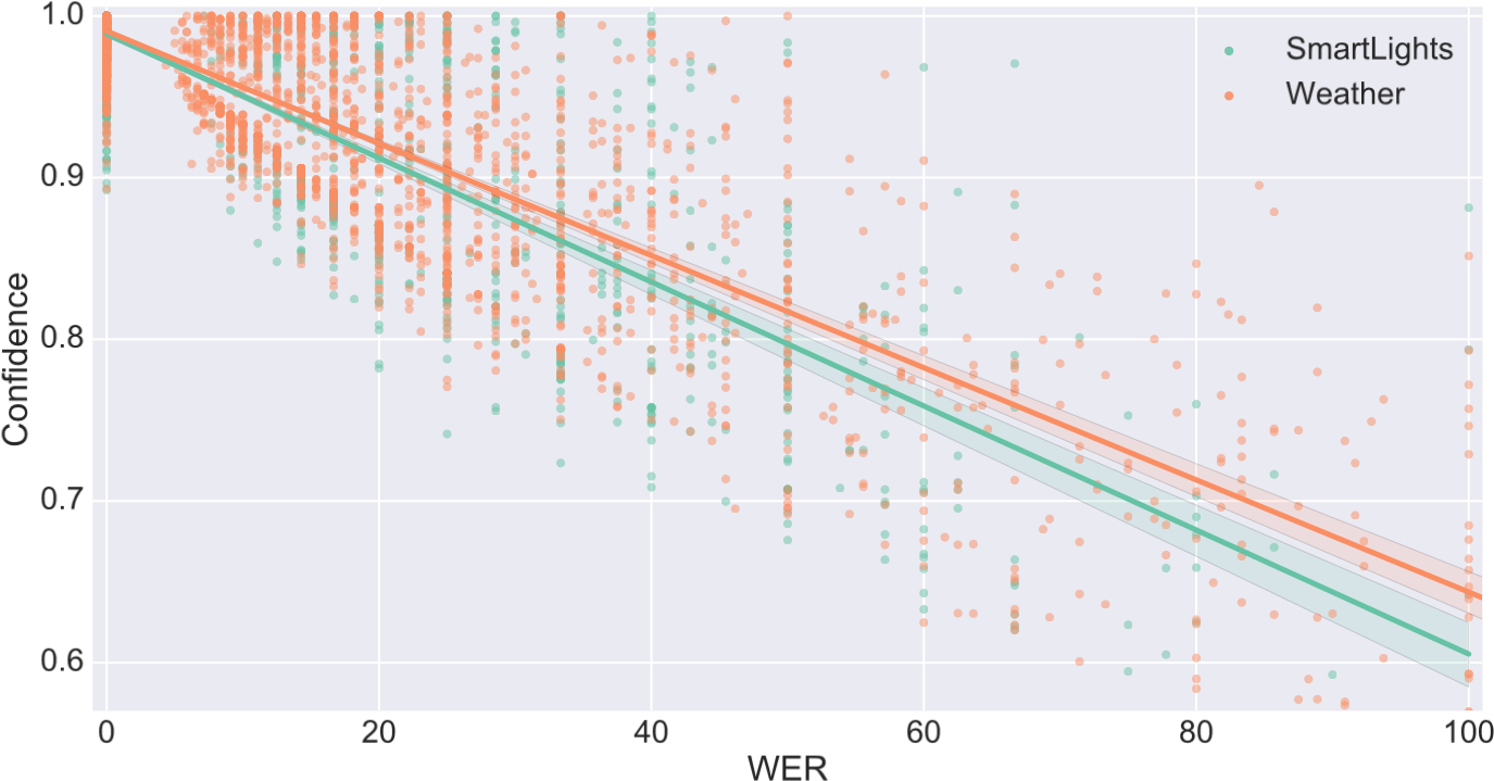
Figure 8: Scatter plot of sentence-level confidence scores against word error rate. Each point represents a sentence from the test set of one of the two assistants, while the lines are obtained through a linear regression. The confidence score is correlated with the word error rate.
5.1.1 Crowdsourcing
Crowdsourcing tasks were originally submitted to Amazon Mechanical Turk[9], a widely used platform in non-expert annotations for natural language tasks [51]. While a sufficient number of Englishspeaking contributors can be reached easily, other languages such as French, German or Japanese suffer from a comparatively smaller available crowd. Local crowdsourcing platforms therefore had to be integrated.
A text query generation task consists in generating an example of user query matching a provided set of intent and slots – e.g. the following set: Intent: The user wants to switch the lights on; slot: (bedroom)[room] could result in the generated query “I want lights in the bedroom right now!”. Fixing entity values reduces the task to a sentence generation and removes the need for a slot labeling step, limiting the sources of error. Diversity is enforced by both submitting this task to the widest possible crowd while limiting the number of available tasks per contributor and by selecting large sets of slot values.
Each generated query goes through a validation process taking the form of a second crowdsourcing task, where at least two out of three new contributors must confirm its formulation, spelling, and intent. Majority voting is indeed a simple and straightforward approach for quality assessment in crowdsourcing [19]. A custom dashboard hosted on our servers has been developed to optimize the contributor’s workflow, with clear descriptions of the task. The dashboard also prevents a contributor from submitting a query that does not contain the imposed entity values, with a fuzzy matching rule allowing for inflections in all supported languages (conjugation, plural, gender, compounds, etc.).
5.1.2 Disambiguation
While the previous validation step allows to filter out most spelling and formulation mistakes, it does not always guarantee the correctness of the intent or the absence of spurious entities. Indeed, in a first type of errors, the intent of the query may not match the provided one – e.g. Switch off the lights when the intent SwitchLightOn was required. In a second type of errors, spurious entities may be added by the contributor, so that they are not labeled as such – e.g. “I want lights in the guest bedroom at _60 _right now!” when only bedroom was mentioned in the task specifications. An unlabeled entity has a particularly strong impact on the CRF features in the NLU component, and limits the ability of the LM to generalize. These errors in the training queries must be fixed to achieve a high accuracy of the SLU.
To do so, we perform a 3-fold cross validation of the NLU engine on this dataset. This yields predicted intents and slots for each sentence in the dataset. By repeating this procedure several times, we obtain several predictions for each sentence. We then apply majority voting on these predictions to detect missing slots and wrong intents. Slots may therefore be extended – e.g. (bedroom)[room] → (guest bedroom)[room] in the previous example – or added – (60)[intensity] – and ill-formed queries (with regard to spelling or intent) are filtered-out. 5.2 Evaluation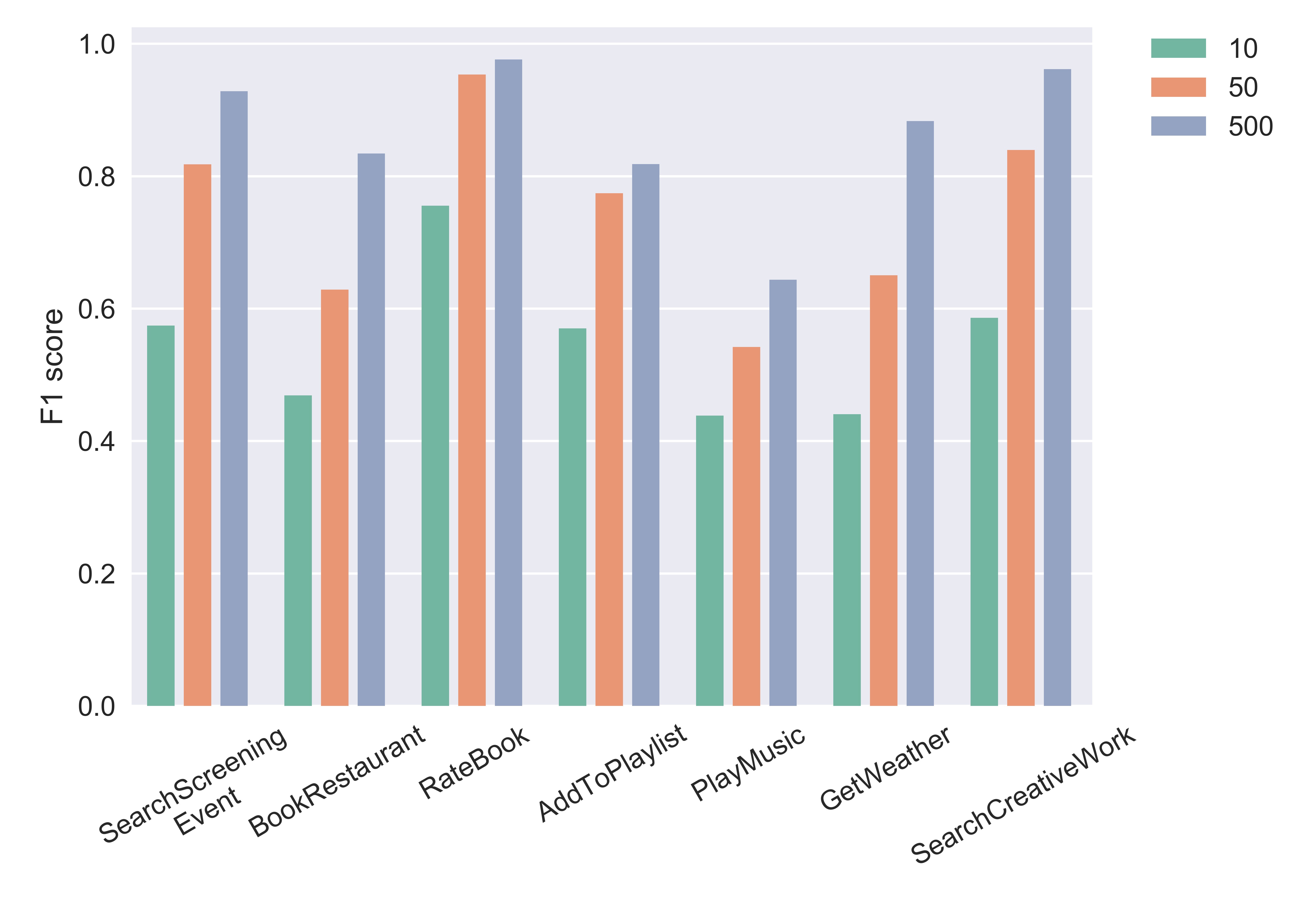
Figure 9: Average F1-score for the slot-filling task for various intents depending on the number of training queries, for 10 (green), 50 (orange), and 500 (blue) queries.
We illustrate the impact of data generation on the SLU performance on the specific case of the slot-filling task in the NLU component. The same in-house open dataset of over 16K crowdsourced query presented in Section 3.3.2 is used. Unsurprisingly, slot-filling performance drastically increases with the number of training samples. The F1-scores averaged over all slots are computed, depending on the number of training queries per intent. An NLU engine has been trained on each individual intent. Training queries are freely available on GitHub[10]. The data has been generated with our data generation pipeline.
Figure 9 shows the influence of the number of training samples on the performance of the slot-filling task of the NLU component. Compared to 10 training queries, the gain in performance with 500 queries is of 32% absolute on average, ranging from 22% for the RateBook intent (from 0.76 to 0.98) to 44% for the GetWeather intent (from 0.44 to 0.88). This gain indeed strongly depends on the intent’s complexity, which is mainly defined by its entities (number of entities, built-in or custom, number of entity values, etc.). While a few tens of training queries might suffice for some simple use cases (such as RateBook), more complicated intents with larger sets of entity values (PlayMusic for instance) require larger training datasets.
While it is easy to manually generate up to 50 queries, being able to come up with hundreds or thousands of diverse formulations of the same intent is nearly impossible. For private-by-design assistants that do not gather user queries, the ability to generate enough queries is key to training efficient machine learning models. Moreover, being able to generate training data allows us to validate the performance of our models before deploying them.
6 Conclusion
In this paper, we have described the design of the Snips Voice Platform, a Spoken Language
Understanding solution that can be embedded in small devices and runs entirely offline. In compliance with the privacy-by-design principle, assistants created through the Snips Voice Platform never send user queries to the cloud and offer state-of-the-art performance. Focusing on the Automatic Speech Recognition and Natural Language Understanding engines, we have described the challenges of embedding high-performance machine learning models on small IoT devices. On the acoustic modeling side, we have shown how small-sized neural networks can be trained that enjoy near state-of-the-art accuracy while running in real-time on small devices. On the language modeling side, we have described how to train the language model of the ASR and the NLU in a consistent way, efficiently specializing them to a particular use case. We have also demonstrated the accuracy of the resulting SLU engine on real-world assistants. Finally, we have shown how sufficient, highquality training data can be obtained without compromising user privacy through a combination of crowdsourcing and machine learning.
We hope that the present paper can contribute to a larger effort towards ever more private and ubiquitous artificial intelligence. Future research directions will include private analytics, allowing to receive privacy-preserving feedback from assistant usage, and federated learning, as a complement to data generation.
Acknowledgments
All of the work presented here has been done closely together with the engineering teams at Snips. We are grateful to the crowd of contributors who regularly work with us on the data generation pipeline. We are indebted to the community of users of the Snips Voice Platform for valuable feedback and contributions.
Appendix: NLU benchmark on an in-house dataset
| Intent Name | Slots | Samples | #Utterances |
|---|---|---|---|
| PlayMusic | album, artist, | I want to hear I want to break free by Queen | 2300 |
| track | on Spotify | ||
| playlist music item | Play the top-5 soul songs | ||
| service sort year genre | Put on John Lennon’s 1980 album | ||
| GetWeather | city, country, | Will it be sunny tomorrow near | 2300 |
| state | North Creek Forest? | ||
| poi time range | How chilly is it here? | ||
| condition temperature spatial relation current location | Should we expect fog in London, UK? | ||
| BookRestaurant | sort | I’d like to eat at a taverna that serves | 2273 |
| party size nb | chili con carne with a party of 10 | ||
| party size descr spatial relation | Make a reservation at a highly rated pub | ||
| city, country | for tonight in Paris within walking distance | ||
| state | from my hotel | ||
| poi restaurant type |
Book an italian place with a parking | ||
| restaurant name cuisine served dish time range facility |
for my grand father and I | ||
| AddToPlaylist | name, artist | Add Diamonds to my roadtrip playlist | 2242 |
| playlist owner playlist music item | Please add Eddy De Pretto’s album | ||
| RateBook | type | Rate the current saga three stars | 2256 |
| name rating unit | Rate Of Mice and Men 5 points out of 6 | ||
| best rating rating value select series | I give the previous essay a four | ||
| SearchCreativeWork | type name | Find the movie named Garden State | 2254 |
| SearchScreeningEvent | object | Which movie theater is playing | 2259 |
| type | The Good Will Hunting nearby? | ||
| name location type | Show me the movie schedule at the | ||
| location name spatial relation time range | Grand Rex tonight |
Table 15: In-house slot-filling dataset summary
| intent | NLU provider | train size | precision | recall | F1-score |
|---|---|---|---|---|---|
| SearchCreativeWork | Luis | 70 2000 |
0.993 1.000 |
0.746 0.995 |
0.849 0.997 |
| Wit | 70 2000 |
0.959 0.974 |
0.569 0.955 |
0.956 0.964 |
|
| API.ai | 70 2000 |
0.915 1.000 |
0.711 0.968 |
0.797 0.983 |
|
| Alexa | 70 2000 |
0.492 0.464 |
0.323 0.375 |
0.383 0.413 |
|
| Snips | 70 2000 |
0.864 0.983 |
0.908 0.976 |
0.885 0.980 |
|
| GetWeather | Luis | 70 2000 |
0.781 0.985 |
0.271 0.902 |
0.405 0.940 |
| Wit | 70 2000 |
0.790 0.847 |
0.411 0.874 |
0.540 0.825 |
|
| API.ai | 70 2000 |
0.666 0.826 |
0.513 0.751 |
0.530 0.761 |
|
| Alexa | 70 2000 |
0.764 0.818 |
0.470 0.701 |
0.572 0.746 |
|
| Snips | 70 2000 |
0.791 0.964 |
0.703 0.926 |
0.742 0.943 |
|
| PlayMusic | Luis | 70 2000 |
0.983 0.816 |
0.265 0.737 |
0.624 0.761 |
| Wit | 70 2000 |
0.677 0.773 |
0.336 0.518 |
0.580 0.655 |
|
| API.ai | 70 2000 |
0.549 0.744 |
0.486 0.701 |
0.593 0.716 |
|
| Alexa | 70 2000 |
0.603 0.690 |
0.384 0.518 |
0.464 0.546 |
|
| Snips | 70 2000 |
0.546 0.876 |
0.482 0.792 |
0.577 0.823 |
Table 16: Precision, recall and F1-score averaged on all slots in an in-house dataset, run in June 2017.
| intent | NLU provider | train size | precision | recall | F1-score |
|---|---|---|---|---|---|
| AddToPlaylist | Luis | 70 2000 |
0.759 0.971 |
0.575 0.938 |
0.771 0.953 |
| Wit | 70 2000 |
0.647 0.862 |
0.478 0.761 |
0.662 0.799 |
|
| API.ai | 70 2000 |
0.830 0.943 |
0.740 0.951 |
0.766 0.947 |
|
| Alexa | 70 2000 |
0.718 0.746 |
0.664 0.704 |
0.667 0.724 |
|
| Snips | 70 2000 |
0.787 0.914 |
0.788 0.891 |
0.785 0.900 |
|
| RateBook | Luis | 70 2000 |
0.993 1.000 |
0.843 0.997 |
0.887 0.999 |
| Wit | 70 2000 |
0.987 0.990 |
0.922 0.950 |
0.933 0.965 |
|
| API.ai | 70 2000 |
0.868 0.976 |
0.830 0.983 |
0.840 0.979 |
|
| Alexa | 70 2000 |
0.873 0.867 |
0.743 0.733 |
0.798 0.784 |
|
| Snips | 70 2000 |
0.966 0.997 |
0.962 0.997 |
0.964 0.997 |
|
| SearchScreeningEvent | Luis | 70 2000 |
0.995 1.000 |
0.721 0.961 |
0.826 0.979 |
| Wit | 70 2000 |
0.903 0.849 |
0.773 0.849 |
0.809 0.840 |
|
| API.ai | 70 2000 |
0.859 0.974 |
0.754 0.959 |
0.800 0.966 |
|
| Alexa | 70 2000 |
0.710 0.695 |
0.515 0.541 |
0.560 0.585 |
|
| Snips | 70 2000 |
0.881 0.965 |
0.840 0.971 |
0.858 0.967 |
|
| BookRestaurant | Luis | 70 2000 |
0.859 0.906 | 0.336 0.891 | 0.473 0.892 |
| Wit | 70 2000 |
0.901 0.841 | 0.436 0.739 | 0.597 0.736 | |
| API.ai | 70 2000 |
0.705 0.874 | 0.548 0.853 | 0.606 0.834 | |
| Alexa | 70 2000 |
0.598 0.760 |
0.364 0.575 |
0.504 0.689 |
|
| Snips | 70 2000 |
0.727 0.919 |
0.700 0.891 |
0.719 0.903 |
Table 17: Precision, recall and F1-score averaged on all slots in an in-house dataset, run in June 2017.
References
- Petar Aleksic, Mohammadreza Ghodsi, Assaf Michaely, Cyril Allauzen, Keith Hall, Brian Roark, David Rybach, and Pedro Moreno. Bringing contextual information to google speech recognition. In Sixteenth Annual Conference of the International Speech Communication Association, 2015.
- Cyril Allauzen, Michael Riley, and Johan Schalkwyk. A generalized composition algorithm for weighted finite-state transducers. In Tenth Annual Conference of the International Speech Communication Association, 2009.
- Cyril Allauzen, Michael Riley, and Johan Schalkwyk. Filters for efficient composition of weighted finite-state transducers. In International Conference on Implementation and Application of Automata, pages 28–38. Springer, 2010.
- Cyril Allauzen, Michael Riley, Johan Schalkwyk, Wojciech Skut, and Mehryar Mohri. Openfst: A general and efficient weighted finite-state transducer library. In International Conference on Implementation and Application of Automata, pages 11–23. Springer, 2007.
- Dzmitry Bahdanau, Jan Chorowski, Dmitriy Serdyuk, Philemon Brakel, and Yoshua Bengio. End-to-end attention-based large vocabulary speech recognition. In Acoustics, Speech and Signal Processing (ICASSP), 2016 IEEE International Conference on, pages 4945–4949. IEEE, 2016.
- Tobias Bocklet, Andreas Maier, Josef G Bauer, Felix Burkhardt, and Elmar Noth. Age and gender recognition for telephone applications based on gmm supervectors and support vector machines. In Acoustics, Speech and Signal Processing, 2008. ICASSP 2008. IEEE International Conference on, pages 1605–1608. IEEE, 2008.
- Tom Bocklisch, Joey Faulker, Nick Pawlowski, and Alan Nichol. Rasa: Open source language understanding and dialogue management. arXiv preprint arXiv:1712.05181, 2017.
- Daniel Braun, Adrian Hernandez-Mendez, Florian Matthes, and Manfred Langen. Evaluating natural language understanding services for conversational question answering systems. In Proceedings of the 18th Annual SIGdial Meeting on Discourse and Dialogue, pages 174–185, 2017.
- Peter F Brown, Peter V Desouza, Robert L Mercer, Vincent J Della Pietra, and Jenifer C Lai. Class-based n-gram models of natural language. Computational linguistics, 18(4):467–479, 1992.
- Ann Cavoukian. Privacy by design. Take the challenge. Information and privacy commissioner of Ontario, Canada, 2009.
- Ciprian Chelba, Dan Bikel, Maria Shugrina, Patrick Nguyen, and Shankar Kumar. Large scale language modeling in automatic speech recognition. arXiv preprint arXiv:1210.8440, 2012.
- Ciprian Chelba, Johan Schalkwyk, Thorsten Brants, Vida Ha, Boulos Harb, Will Neveitt, Carolina Parada, and Peng Xu. Query language modeling for voice search. In Spoken Language Technology Workshop (SLT), 2010 IEEE, pages 127–132. IEEE, 2010.
- Facebook. Language, engine, and tooling for expressing, testing, and evaluating composable language rules on input strings. GitHub repository, https://github.com/facebook/ duckling, 2017.
- Alex Graves, Abdel-rahman Mohamed, and Geoffrey Hinton. Speech recognition with deep recurrent neural networks. In Acoustics, speech and signal processing (icassp), 2013 ieee international conference on, pages 6645–6649. IEEE, 2013.
- Dilek Hakkani-Tür, Frédéric Béchet, Giuseppe Riccardi, and Gokhan Tur. Beyond asr 1best: Using word confusion networks in spoken language understanding. Computer Speech & Language, 20(4):495–514, 2006.
- Melinda Hamill, Vicky Young, Jennifer Boger, and Alex Mihailidis. Development of an automated speech recognition interface for personal emergency response systems. Journal of NeuroEngineering and Rehabilitation, 6(1):26, 2009.
- Geoffrey Hinton, Li Deng, Dong Yu, George E Dahl, Abdel-rahman Mohamed, Navdeep Jaitly, Andrew Senior, Vincent Vanhoucke, Patrick Nguyen, Tara N Sainath, et al. Deep neural networks for acoustic modeling in speech recognition: The shared views of four research groups. IEEE Signal Processing Magazine, 29(6):82–97, 2012.
- Axel Horndasch, Caroline Kaufhold, and Elmar Nöth. How to add word classes to the kaldi speech recognition toolkit. In International Conference on Text, Speech, and Dialogue, pages 486–494. Springer, 2016.
- Panagiotis G Ipeirotis, Foster Provost, Victor S Sheng, and Jing Wang. Repeated labeling using multiple noisy labelers. Data Mining and Knowledge Discovery, 28(2):402–441, 2014.
- Hui Jiang. Confidence measures for speech recognition: A survey. Speech communication, 45(4):455–470, 2005.
- Slava Katz. Estimation of probabilities from sparse data for the language model component of a speech recognizer. IEEE transactions on acoustics, speech, and signal processing, 35(3):400– 401, 1987.
- Chanwoo Kim, Ananya Misra, Kean Chin, Thad Hughes, Arun Narayanan, Tara Sainath, and Michiel Bacchiani. Generation of large-scale simulated utterances in virtual rooms to train deep-neural networks for far-field speech recognition in google home. Proc. INTERSPEECH. ISCA, 2017.
- Anjishnu Kumar, Arpit Gupta, Julian Chan, Sam Tucker, Bjorn Hoffmeister, and Markus Dreyer. Just ask: Building an architecture for extensible self-service spoken language understanding. arXiv preprint arXiv:1711.00549, 2017.
- John Lafferty, Andrew McCallum, and Fernando CN Pereira. Conditional random fields: Probabilistic models for segmenting and labeling sequence data. 2001.
- Marc Langheinrich. Privacy by design—principles of privacy-aware ubiquitous systems. In International conference on Ubiquitous Computing, pages 273–291. Springer, 2001.
- Benjamin Lecouteux, Michel Vacher, and François Portet. Distant speech recognition in a smart home: Comparison of several multisource asrs in realistic conditions. In Interspeech 2011 Florence, pages 2273–2276, 2011.
- Percy Liang. Semi-supervised learning for natural language. PhD thesis, Massachusetts Institute of Technology, 2005.
- Lidia Mangu, Eric Brill, and Andreas Stolcke. Finding consensus in speech recognition: word error minimization and other applications of confusion networks. Computer Speech & Language, 14(4):373–400, 2000.
- Nicholas D Matsakis and Felix S Klock II. The rust language. In ACM SIGAda Ada Letters, volume 34, pages 103–104. ACM, 2014.
- Grégoire Mesnil, Yann Dauphin, Kaisheng Yao, Yoshua Bengio, Li Deng, Dilek Hakkani-Tur, Xiaodong He, Larry Heck, Gokhan Tur, Dong Yu, et al. Using recurrent neural networks for slot filling in spoken language understanding. IEEE/ACM Transactions on Audio, Speech, and Language Processing, 23(3):530–539, 2015.
- Grégoire Mesnil, Xiaodong He, Li Deng, and Yoshua Bengio. Investigation of recurrent-neuralnetwork architectures and learning methods for spoken language understanding. In Interspeech, pages 3771–3775, 2013.
- Tomas Mikolov, Kai Chen, Greg Corrado, and Jeffrey Dean. Efficient estimation of word representations in vector space. arXiv preprint arXiv:1301.3781, 2013.
- Abdel-rahman Mohamed, George E Dahl, and Geoffrey Hinton. Acoustic modeling using deep belief networks. IEEE Transactions on Audio, Speech, and Language Processing, 20(1):14–22, 2012.
- Mehryar Mohri, Fernando Pereira, and Michael Riley. Weighted finite-state transducers in speech recognition. Departmental Papers (CIS), page 11, 2001.
- Mehryar Mohri, Fernando Pereira, and Michael Riley. Speech recognition with weighted finite-state transducers. In Springer Handbook of Speech Processing, pages 559–584. Springer, 2008.
- Josef Robert Novak, Nobuaki Minematsu, and Keikichi Hirose. Phonetisaurus: Exploring grapheme-to-phoneme conversion with joint n-gram models in the wfst framework. Natural Language Engineering, 22(6):907–938, 2016.
- Olutobi Owoputi, Brendan O’Connor, Chris Dyer, Kevin Gimpel, Nathan Schneider, and Noah A Smith. Improved part-of-speech tagging for online conversational text with word clusters. Association for Computational Linguistics, 2013.
- Vassil Panayotov, Guoguo Chen, Daniel Povey, and Sanjeev Khudanpur. Librispeech: an asr corpus based on public domain audio books. In Acoustics, Speech and Signal Processing (ICASSP), 2015 IEEE International Conference on, pages 5206–5210. IEEE, 2015.
- Vijayaditya Peddinti, Daniel Povey, and Sanjeev Khudanpur. A time delay neural network architecture for efficient modeling of long temporal contexts. In Sixteenth Annual Conference of the International Speech Communication Association, 2015.
- Vijayaditya Peddinti, Yiming Wang, Daniel Povey, and Sanjeev Khudanpur. Low latency acoustic modeling using temporal convolution and lstms. IEEE Signal Processing Letters, 25(3):373–377, 2018.
- Bastian Pfleging, Stefan Schneegass, and Albrecht Schmidt. Multimodal interaction in the car: combining speech and gestures on the steering wheel. In Proceedings of the 4th International Conference on Automotive User Interfaces and Interactive Vehicular Applications, pages 155– 162. ACM, 2012.
- Daniel Povey, Arnab Ghoshal, Gilles Boulianne, Lukas Burget, Ondrej Glembek, Nagendra Goel, Mirko Hannemann, Petr Motlicek, Yanmin Qian, Petr Schwarz, et al. The kaldi speech recognition toolkit. In IEEE 2011 workshop on automatic speech recognition and understanding, number EPFL-CONF-192584. IEEE Signal Processing Society, 2011.
- Daniel Povey, Vijayaditya Peddinti, Daniel Galvez, Pegah Ghahremani, Vimal Manohar, Xingyu Na, Yiming Wang, and Sanjeev Khudanpur. Purely sequence-trained neural networks for asr based on lattice-free mmi. In Interspeech, pages 2751–2755, 2016.
- Rohit Prabhavalkar, Ouais Alsharif, Antoine Bruguier, and Lan McGraw. On the compression of recurrent neural networks with an application to lvcsr acoustic modeling for embedded speech recognition. In Acoustics, Speech and Signal Processing (ICASSP), 2016 IEEE International Conference on, pages 5970–5974. IEEE, 2016.
- Christian Raymond and Giuseppe Riccardi. Generative and discriminative algorithms for spoken language understanding. In Eighth Annual Conference of the International Speech Communication Association, 2007.
- Marta Sabou, Kalina Bontcheva, and Arno Scharl. Crowdsourcing research opportunities:
lessons from natural language processing. In Proceedings of the 12th International Conference on Knowledge Management and Knowledge Technologies, page 17. ACM, 2012.
- Johan Schalkwyk, Doug Beeferman, Françoise Beaufays, Bill Byrne, Ciprian Chelba, Mike Cohen, Maryam Kamvar, and Brian Strope. “your word is my command”: Google search by voice: a case study. In Advances in speech recognition, pages 61–90. Springer, 2010.
- Snips Team. Rustling, Rust implementation of Duckling. GitHub repository, https://github.
com/snipsco/rustling, 2018.
- Snips Team. Snips NLU rust, Snips NLU Rust implementation. GitHub repository, https: //github.com/snipsco/snips-nlu-rs, 2018.
- Snips Team. Snips NLU, Snips Python library to extract meaning from text. GitHub repository, https://github.com/snipsco/snips-nlu, 2018.
- Rion Snow, Brendan O’Connor, Daniel Jurafsky, and Andrew Y Ng. Cheap and fast—but is it good?: evaluating non-expert annotations for natural language tasks. In Proceedings of the conference on empirical methods in natural language processing, pages 254–263. Association for Computational Linguistics, 2008.
- Maksim Tkachenko and Andrey Simanovsky. Named entity recognition: Exploring features. In KONVENS, pages 118–127, 2012.
- Gökhan Tür, Anoop Deoras, and Dilek Hakkani-Tür. Semantic parsing using word confusion networks with conditional random fields. In INTERSPEECH, pages 2579–2583, 2013.
- Ye-Yi Wang and Alex Acero. Discriminative models for spoken language understanding. In Ninth International Conference on Spoken Language Processing, 2006.
- Yiming Wang, Vijayaditya Peddinti, Hainan Xu, Xiaohui Zhang, Daniel Povey, and Sanjeev Khudanpur. Backstitch: Counteracting finite-sample bias via negative steps. NIPS (submitted), 2017.
- Wayne Xiong, Jasha Droppo, Xuedong Huang, Frank Seide, Mike Seltzer, Andreas Stolcke, Dong Yu, and Geoffrey Zweig. Achieving human parity in conversational speech recognition. arXiv preprint arXiv:1610.05256, 2016.
- Haihua Xu, Daniel Povey, Lidia Mangu, and Jie Zhu. Minimum bayes risk decoding and system combination based on a recursion for edit distance. Computer Speech & Language, 25(4):802–828, 2011.
- Roman V Yampolskiy and Venu Govindaraju. Behavioural biometrics: a survey and classification. International Journal of Biometrics, 1(1):81–113, 2008.
- Dong Yu, Jinyu Li, and Li Deng. Calibration of confidence measures in speech recognition. IEEE Transactions on Audio, Speech, and Language Processing, 19(8):2461–2473, 2011.
- https://www.voicebot.ai/2018/03/07/new-voicebot-report-says-nearly-20-u-sadults-smart-speakers/
- In French: https://www.cnil.fr/fr/enceintes-intelligentes-des-assistants-vocauxconnectes-votre-vie-privee
- https://www.eugdpr.org/ ↑
- https://console.snips.ai ↑
- http://www.openslr.org/11/ ↑
- BILOU is a standard acronym referring to the possible positions of a symbol in a sequence: Beginning, Inside, Last, Outside, Unit. ↑
- Complete list available here: https://github.com/snipsco/snips-nlu-ontology 8
https://github.com/snipsco/nlu-benchmark - See footnote 8 ↑
- https://www.mturk.com/
- https://github.com/snipsco/nlu-benchmark

若有收获,就点个赞吧
0 人点赞
