前言
AlexNet是由Alex Krizhevsky等人于2012年提出的一个开创性的卷积神经网络。本文参考Alex的两篇论文ImageNet Classification with Deep Convolutional以及One weird trick for parallelizing convolutional neural networks,详细介绍了模型了复现步骤和其PyTorch的实现代码。这里前者我将其称为AlextNetV1, 后者称为AlexNetV2。
完整代码
完整代码,训练日志和模型文件请参考:
https://github.com/ethanyanjiali/deep-vision/tree/master/CNNs/imagenet-2012/pytorch#alexnet
网络结构
AlexNetV1
由于当年GPU资源不足,V1采取了双塔的方案。具体双塔的意思是将一张图像分割为两部分,并使用两组GPU分别对其不同部分提取特征,然后再将结果整合起来。不过由于目前单个GPU的容量完全足以支撑起整个模型,本文采取了单塔方案进行复现,并因此将参数提高了一倍。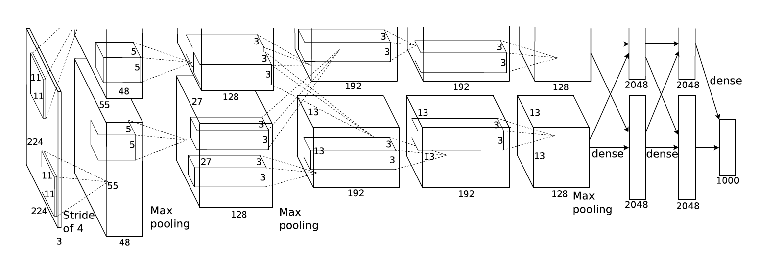
AlexNet1的结构可谓是教科书一般的卷积深度神经网络:卷积层,激活层,正则化层加上池化层四层一组构成一个特征提取单元,多个特征提取单元的串联构成一个特征提取器,或者叫做编码器(Encoder)。该特征提取器的目标就是将原始的RGB数据提取成一个特征向量。在特征提取器之后,由多层全连接层(Fully Conntected Layer, Dense Layer)配合随机选择层(Dropout)又构成一个分类单元,多个分类单元又可以组成一个分类器。分类器的作用是将特征向量最终映射到目标训练值上。这奠定了之后很多神经网络的基础结构。虽然不同的网络会对某一层稍有不同的改动,比如改用Batch Normalization或者Average Pooling,但是万变不离其宗。下面贴出完整的网络结构代码,然后我再对每一部分详细解释:
# coding: utf-8import torchimport torch.nn as nn# [1] ImageNet Classification with Deep Convolutional Neural Networks# https://papers.nips.cc/paper/4824-imagenet-classification-with-deep-convolutional-neural-networks.pdf# [2] http://cs231n.github.io/convolutional-networks# [3] https://prateekvjoshi.com/2016/04/05/what-is-local-response-normalization-in-convolutional-neural-networks/class AlexNetV1(nn.Module):def __init__(self):super(AlexNetV1, self).__init__()# formula# [conv layer]# output_size = (input_size - kernel_size + 2 * padding) / stride + 1# padding = ((output_size - 1) * stride) + kernel_size - input_size) / 2# [pooling layer]# output_size = (input_size - kernel_size) / stride + 1# where input_size and output_size are the square image side lengthself.features = nn.Sequential(# "The first convolutional layer filters the 224×224×3 input image with# 96 kernels of size 11×11×3 with a stride of 4 pixels."[1]# Also from [1]Fig.2, next layer is 55x55x48, output channels is 48. (I use 96=2x48 here)# hence padding = ((55 - 1) * 4 + 11 - 224) / 2 = 2# to verify, output = (224 - 11 + 2 * 2) / 4 + 1 = 55nn.Conv2d(3, 96, 11, stride=4, padding=2),# The ReLU non-linearity is applied to the output of every convolutional# and fully-connected layer.nn.ReLU(inplace=True),# "The second convolutional layer takes as input the (response-normalized# and pooled) output of the first convolutional layer"nn.LocalResponseNorm(96),# From Fig.2 in [1], there's a maxpooling layer after first conv layer# Also from Fig.2 in [1], the pooling reduces dimension from 55x55 to 27x27# hence it's likely that they uses overlapping pooling kernel=3, stride=2# to verify, output_size = (55 - 3) / 2 + 1 = 27nn.MaxPool2d(3, 2),# "The second convolutional layer takes ... with 256 kernels of size 5 × 5 × 48."[1]# From Fig.2 in [1], output channels is 128. (I use 256=2x128 here)# To keep dimension same as 27, we can infer that stride = 2, padding = 1# output_size = (27 - 5 + 2 * 2) / 1 + 1 = 27nn.Conv2d(96, 256, 5, stride=1, padding=2),nn.ReLU(inplace=True),# "The third convolutional layer has 384 kernels of size 3 × 3 ×# 256 connected to the (normalized, pooled) outputs of the second convolutional layer"[1]# Since the output of second layer is 256, the normalized layer input should be 256 here as wellnn.LocalResponseNorm(256),# From Fig.2 in [1], there's a maxpooling layer after second conv layer# Also from Fig.2 in [1], the pooling reduces dimension from 27x27 to 13x13# similar to last one, output_size = (27 - 3) / 2 + 1 = 13nn.MaxPool2d(3, 2),# "The third, fourth, and fifth convolutional layers are connected to one another# without any intervening pooling or normalization layers"[1]# Also from Fig.2 in [1], next layer is 13x13x192, and it uses a kernel size of 3.# (I use 384=2x192 here)# to keep dimension same as 13, we can infer that stride = 1, padding = 1# output_size = (13 - 3 + 2 * 1) / 1 + 1 = 13nn.Conv2d(256, 384, 3, stride=1, padding=1),nn.ReLU(inplace=True),# same as last conv layer# output_size = (13 - 3 + 2 * 1) / 1 + 1 = 13# (I use 384=2x192 here)nn.Conv2d(384, 384, 3, stride=1, padding=1),nn.ReLU(inplace=True),# From Fig.2 in [1], the output channels drop to 128# (I use 256=2x128 here)# output_size = (13 - 3 + 2 * 1) / 1 + 1 = 13nn.Conv2d(384, 256, 3, stride=1, padding=1),nn.ReLU(inplace=True),# there's another pooling layer after 5th conv layer from Fig.2 in [1]# output_size = (13 - 3) / 2 + 1 = 6nn.MaxPool2d(3, 2),)self.classifier = nn.Sequential(# "We use dropout in the first two fully-connected layers of Figure 2.# Without dropout, our network exhibits substantial overfitting.# Dropout roughly doubles the number of iterations required to converge."[1]# "...consists of setting to zero the output of each hidden neuron with probability 0.5"[1]nn.Dropout(p=0.5),# From Fig.2 in [1], the frist FC layer has 4096 (2x2048) activationsnn.Linear(6 * 6 * 256, 4096),nn.ReLU(inplace=True),nn.Dropout(p=0.5),# From Fig.2 in [1], the second FC layer also has 4096 activationsnn.Linear(4096, 4096),nn.ReLU(inplace=True),# "The output of the last fully-connected layer is fed to a 1000-way softmax which produces# a distribution over the 1000 class labels."[1]nn.Linear(4096, 1000),# There's no softmax here because we use CrossEntropyLoss which already includes Softmax# https://discuss.pytorch.org/t/vgg-output-layer-no-softmax/9273/5)def forward(self, x):x = self.features(x)# flatten the output from conv layers, but keep batch sizex = x.view(x.size(0), 6 * 6 * 256)x = self.classifier(x)return x
在init函数中,我们定好需要使用的网络模块,然后再在forward函数中定义他们的调用顺序。PyTorch通过python的执行顺序来动态定义图,相比TensorFlow简单了许多。
self.features = nn.Sequential(nn.Conv2d(3, 96, 11, stride=4, padding=2),nn.ReLU(inplace=True),nn.LocalResponseNorm(96),nn.MaxPool2d(3, 2),nn.Conv2d(96, 256, 5, stride=1, padding=2),nn.ReLU(inplace=True),nn.LocalResponseNorm(256),nn.MaxPool2d(3, 2),nn.Conv2d(256, 384, 3, stride=1, padding=1),nn.ReLU(inplace=True),nn.Conv2d(384, 384, 3, stride=1, padding=1),nn.ReLU(inplace=True),nn.Conv2d(384, 256, 3, stride=1, padding=1),nn.ReLU(inplace=True),nn.MaxPool2d(3, 2),)
这里我们可以清晰的看见,整个网络有两大部分,features就是特征提取器,classifier就是分类器。这里参数的定义都是按照文中所给参数x2 (由于双塔变单塔)。如上,在features部分,参考论文中图2的展示,每一个卷积层后都使用ReLu非线性函数。按照作者的意思,前两个卷积层后还附带LRN以提高网络性能。该网络先由一个11×11的卷积层开始,接着一个池化层降低维数,再用一个5×5的卷积层和一个池化层。之后,接上三个过滤器为3×3的小卷积层,并再次池化,特征提取部分便完成了。这里基本的思路是底层卷积层用大卷积核提取更广阔的范围,高层卷积层用小卷积核来保证细节的提取。然而在后世的网络中我们发现,小卷积核其实更有效率。AlexNet相比之后的各类神经网络全是不能算是深度神经网络,但启发了之后VGG和GoogLeNet团队继续加深网络的想法。
特征提取完毕后,我们使用提取的特征输入全连接层进行分类
self.classifier = nn.Sequential(nn.Dropout(p=0.5),nn.Linear(6 * 6 * 256, 4096),nn.ReLU(inplace=True),nn.Dropout(p=0.5),nn.Linear(4096, 4096),nn.ReLU(inplace=True),nn.Linear(4096, 1000),)
这里作者在每个线性层之前都加入了Dropout层,通过随机关闭一些Activation通道,来达到regularization降低过度拟合的风险。第一个线性层的输入是上面我们特征提取的输出,而之后都是4096。最后一个线性层输出1000个分类。这里并没有加入Softmax,因为之后我们的Optimizer将添加这一部分。
前向传播部分就非常简单了,将我们之前定义好的特征提取和分类器连接起来就好了,只是中间需要将特征提取的输出展开铺平,方便线性层使用。
def forward(self, x):x = self.features(x)x = x.view(x.size(0), 6 * 6 * 256)x = self.classifier(x)return x
AlexNetV2
在V1出世不久,Alex又提出了一个改进版网络,改进版同样取消了双塔的操作,合并到单塔,同时调整了一些参数以提高单GPU下网络的性能。这里我将其叫做AlexNetV2.
首先贴出完整网络结构代码:
# coding: utf-8import torchimport torch.nn as nnimport torch.nn.functional as Func# can use the below import should you choose to initialize the weights of your Netimport torch.nn.init as Init# [1] One weird trick for parallelizing convolutional neural networks https://arxiv.org/pdf/1404.5997.pdfclass AlexNetV2(nn.Module):'''This implements the network from the second version of AlexNet'''def __init__(self):super(AlexNetV2, self).__init__()# "In detail, the single-column model has 64, 192, 384, 384, 256 filters# in the five convolutional layers, respectivel"[1]# "It has the same number of layers as the two-tower model, and the# (x, y) map dimensions in each layer are equivalent to# the (x, y) map dimensions in the two-tower model.# The minor difference in parameters and connections# arises from a necessary adjustment in the number of# kernels in the convolutional layers, due to the unrestricted# layer-to-layer connectivity in the single-tower model."[1]# According to the above, I just need to change the # of output channels# Please refer to ./alexnet1 for detailed calculationself.features = nn.Sequential(nn.Conv2d(3, 64, 11, stride=4, padding=2),nn.ReLU(inplace=True),# Later in the VGG paper, it demonstrated that LRN is not necessary# Hence most of AlexNet implementation doesn't include LRN# However, for study purpose, I still added this layernn.LocalResponseNorm(64),nn.MaxPool2d(3, 2),nn.Conv2d(64, 192, 5, stride=1, padding=2),nn.ReLU(inplace=True),nn.LocalResponseNorm(192),nn.MaxPool2d(3, 2),nn.Conv2d(192, 384, 3, stride=1, padding=1),nn.ReLU(inplace=True),nn.Conv2d(384, 384, 3, stride=1, padding=1),nn.ReLU(inplace=True),nn.Conv2d(384, 256, 3, stride=1, padding=1),nn.ReLU(inplace=True),nn.MaxPool2d(3, 2),)self.classifier = nn.Sequential(# This part is same with ./alexnet 1 as mentioned abovenn.Dropout(p=0.5),nn.Linear(6 * 6 * 256, 4096),nn.ReLU(inplace=True),nn.Dropout(p=0.5),nn.Linear(4096, 4096),nn.ReLU(inplace=True),nn.Linear(4096, 1000),# "Another difference is that instead of a softmax# final layer with multinomial logistic regression# cost, this model’s final layer has 1000 independent logistic# units, trained to minimize cross-entropy"[1])def forward(self, x):x = self.features(x)# flatten the output from conv layers, but keep b∏atch sizex = x.view(x.size(0), 6 * 6 * 256)x = self.classifier(x)return x
可以看出,基本的网络结构是和V1非常相似的,同样是5个卷积层和相应的一些LRN及Maxpooling池化层。在权重初始化部分也同样有相同的限制。
训练代码
这里贴出训练代码中关键部分,完整训练代码请参考文首的Github Repo中train.py。
https://github.com/ethanyanjiali/deep-vision/tree/master/CNNs/imagenet-2012/pytorch#alexnet
https://github.com/ethanyanjiali/deep-vision/tree/master/CNNs/imagenet-2012/pytorch/train.py#L26
transform = transforms.Compose([# "Therefore, we down-sampled the images to a fixed resolution of 256 × 256" alexnet1.[1]Rescale(256),RandomHorizontalFlip(0.5),RandomCrop(224),ToTensor(),])batch_size = 128# instantiate the neural networknet = AlexNetV1()# define the loss function using CrossEntropyLosscriterion = nn.CrossEntropyLoss()# define the params updating function using SGDoptimizer = optim.SGD(net.parameters(),lr=0.01,momentum=0.9,weight_decay=0.0005,)scheduler = optim.lr_scheduler.ReduceLROnPlateau(optimizer,factor=0.1,mode="max",)
在数据预处理transform部分,我首先将图片缩放到256的正方形,然后做了一些数据提升(Data augmentation)的处理,比如将图片随机水平方向翻转,并且在256的区域中随机取得大小为224×224的子区域用作训练。最后一步是将numpy数据转成PyTorch所要求的Tensor数据结构。数据提升看似简单,但实际训练中对训练效果有这至关重要的影响。
训练时,采用了mini-batch方式。batch大小我选了128,如果你不是使用16G GPU的话,需要加大或者减小这个数字,防止内存不够的情况。损失函数就是PyTorch自带的CrossEntropy,注意该函数已经包含了Softmax,所以不要在网络中重复添加,否则无法计算正确的loss。优化器部分就是经典的stochastic gradient descent,这里参数的定义也是按照论文中所述。学习率调整器(learing rate scheduler)部分是我后面加入的,一开始我是手动调整的,之后我使用了平原下降策略(ReduceLROnPlateau),在top1准确率10个epoch还未提升的情况下降学习率降为10%。
结论
AlexNet虽然在性能和体积上都不占优势,在实际生产环境中也很少使用,但其奠定了很多深度神经网络的经典结构,通过对AlexNet的学习,我们能够一瞥CNN历史的进程,对之后学习其他网络打下良好的基础。AlexNet中很多参数的选择也都是经验得来,并无太多理论支持,但是往往一个参数的不同就会导致结果大相径庭。比如网络结构中卷积核的大小,或者训练时学习率,这也体现了深度神经网络调参的重要性。

若有收获,就点个赞吧
0 人点赞
