梯度下降优化算法综述

这篇文章探讨了许多最流行的基于梯度的优化算法实际上是有效的。
注意: 如果你正在寻找一篇评论论文，这篇博客文章也是关于 arXiv 的文章。
更新 09.02.2018: 添加 AMSGrad。
更新 24.11.2017: 本文中的大部分内容现在也可以作为幻灯片提供。
更新 15.06.2017: 添加了 AdaMax 和 Nadam 的衍生产品。
更新 21.0 6.16: 此帖子已发布至黑客新闻。讨论提供了一些相关工作和其他技术的有趣的指针。

目录:

• 梯度下降变量
  • 批量梯度下降
  • 随机梯度下降
  • 小批量梯度下降
• 挑战
• 梯度下降优化算法
  • 动量
  • 加速梯度
  • Adagrad
  • 阿德达塔
  • RMSprop
  • 亚当
  • AdaMax
  • 那达慕
  • AMSGrad
  • 算法可视化
  • 选择哪个优化器？
• SGD 的并行化和分发
  • 霍格菲尔德!
  • 倾盆大雨
  • SGD 的延迟容忍算法
  • TensorFlow
  • 弹性平均 SGD
• 优化 SGD 的附加策略
  • 洗牌与课程学习
  • 批量标准化
  • 提前停车
  • 梯度噪声
• 结论
• 参考资料

梯度下降算法是进行优化的最流行的算法之一，也是迄今为止优化神经网络的最常见的方法。与此同时，每个最先进的深度学习库都包含优化梯度下降的各种算法的实现 (例如 lasagne 、 caffe 和 keras 的文档)。然而，这些算法通常被用作黑盒优化器，因为很难对它们的优缺点进行实际解释。
这篇博客文章旨在为你提供优化梯度下降的不同算法的行为的直觉，这将有助于你使用它们。我们首先来看一下梯度下降的不同变体。然后，我们将简要总结培训过程中的挑战。随后，我们将介绍最常见的优化算法，展示它们解决这些挑战的动机，以及这将如何导致它们更新规则的推导。我们还将简要介绍在并行和分布式环境中优化梯度下降的算法和体系结构。最后，我们将考虑有助于优化梯度下降的附加策略。
Gradient descent is a way to minimize an objective function J(θ)J(θ) parameterized by a model’s parameters θ∈Rdθ∈Rd by updating the parameters in the opposite direction of the gradient of the objective function ∇θJ(θ)∇θJ(θ) w.r.t. to the parameters. The learning rate ηηdetermines the size of the steps we take to reach a (local) minimum. In other words, we follow the direction of the slope of the surface created by the objective function downhill until we reach a valley. If you are unfamiliar with gradient descent, you can find a good introduction on optimizing neural networks here.

梯度下降变量

梯度下降有三种变体，它们与我们用来计算目标函数梯度的数据不同。根据数据量，我们在参数更新的准确性和执行更新所需的时间之间进行权衡。

Batch gradient descent

Vanilla gradient descent, aka batch gradient descent, computes the gradient of the cost function w.r.t. to the parameters θθ for the entire training dataset:
θ=θ−η⋅∇θJ(θ)θ=θ−η⋅∇θJ(θ).
由于我们需要计算整个数据集的梯度来执行一次更新，批量梯度下降可能非常缓慢，对于不适合内存的数据集来说也是棘手的。批量梯度下降也不允许我们在线更新我们的模型，即动态更新新的例子。
在代码中，批量梯度下降看起来是这样的:

for i in range(nb_epochs):
  params_grad = evaluate_gradient(loss_function, data, params)
  params = params - learning_rate * params_grad

对于预定义的周期数，我们首先计算整个数据集 w.r.t.的损失函数的梯度向量参数。我们的参数向量参数。请注意，最先进的深度学习库提供了自动区分功能，可以有效地计算梯度 w.r.t.一些参数。如果你自己推导梯度，那么梯度检查是一个好主意。(有关如何正确检查渐变的一些伟大提示，请参见这里。))
然后，我们用决定我们执行的更新有多大的学习率，在梯度的相反方向更新我们的参数。保证批量梯度下降收敛到凸误差曲面的全局最小值，收敛到非凸曲面的局部最小值。

随机梯度下降

相反，随机梯度下降 (SGD) 对每个训练示例 x (i) 和标签 y (i) 执行参数更新:
θ=θ−η⋅∇θJ(θ;x(i);y(i))θ=θ−η⋅∇θJ(θ;x(i);y(i)).
批量梯度下降对大型数据集执行冗余计算，因为它在每次参数更新之前为类似示例重新计算梯度。SGD 通过一次执行一次更新来消除这种冗余。因此，它通常速度更快，也可以用于在线学习。
SGD 以很高的方差执行频繁更新，导致目标函数像图 1 中那样波动很大。
图片 1: SGD 波动 (来源: 维基百科)
当批量梯度下降收敛到参数所在流域的最小值时，SGD 的波动一方面使它能够跳到新的更好的局部最小值。另一方面，由于 SGD 将继续过度拍摄，这最终使收敛复杂化到精确的最小值。然而，当我们慢慢降低学习率时，SGD 显示出与批梯度下降相同的收敛行为, 对于非凸和凸优化，几乎可以肯定地收敛到局部或全局最小值。
它的代码片段只是在训练示例上添加了一个循环，并评估了梯度 w.r.t.每个例子。请注意，我们在本节中解释的每个时代洗牌训练数据。

for i in range(nb_epochs):
  np.random.shuffle(data)
  for example in data:
    params_grad = evaluate_gradient(loss_function, example, params)
    params = params - learning_rate * params_grad

小批量梯度下降

小批量梯度下降最终兼顾了这两个方面的优点，并对每一个小批量 nn 训练示例执行更新:
θ=θ−η⋅∇θJ(θ;x(i:i+n);y(i:i+n))θ=θ−η⋅∇θJ(θ;x(i:i+n);y(i:i+n)).
这样，a) 减少了参数更新的方差，使得收敛更加稳定; b) 可以利用最先进的深度学习库中常见的高度优化的矩阵优化来计算梯度 w r. t.非常高效的迷你批次。常见的小批量尺寸在 50 到 256 之间，但对于不同的应用可能会有所不同。小批量梯度下降通常是训练神经网络时选择的算法，当使用小批量时，通常也使用术语 SGD。注意: 在本帖子的其余部分中，在对 SGD 的修改中, we leave out the parameters x(i:i+n);y(i:i+n)x(i:i+n);y(i:i+n) for simplicity.
在代码中，我们现在迭代大小为 50 的小批量，而不是迭代示例:

for i in range(nb_epochs):
  np.random.shuffle(data)
  for batch in get_batches(data, batch_size=50):
    params_grad = evaluate_gradient(loss_function, batch, params)
    params = params - learning_rate * params_grad

挑战

然而，香草小批量梯度下降并不能保证良好的收敛，但它提供了一些需要解决的挑战:

• 选择一个合适的学习率是很困难的。太小的学习率会导致收敛缓慢，而太大的学习率会阻碍收敛，并导致损失函数在最小值附近波动，甚至发散。
• 学习率时间表 [1] 尝试通过退火等方式调整培训期间的学习率, 即根据预定义的时间表或当时代之间的目标变化低于阈值时降低学习率。然而，这些时间表和阈值必须事先定义，因此无法适应数据集的特征 [2]。
• 此外，所有参数更新都适用相同的学习率。如果我们的数据是稀疏的，并且我们的特征具有非常不同的频率，我们可能不想在相同的程度上更新所有的特征，而是对很少出现的特征执行更大的
• 最小化神经网络常见的高度非凸误差函数的另一个关键挑战是避免陷入其众多次优局部最小值。Dau等人 [3] 认为，困难实际上不是来自局部最小值，而是来自鞍点，即一个维度向上倾斜而另一个维度向下倾斜的点。这些鞍点通常被相同误差的平台包围，这使得 SGD 很难逃脱，因为在所有维度中梯度都接近零。

  梯度下降优化算法

  在下面，我们将概述一些深度学习社区广泛使用的算法来应对上述挑战。我们不会讨论在实践中计算高维数据集不可行的算法，例如二阶方法，如牛顿法。

  动量

  SGD 在浏览峡谷时遇到了困难，即在一个维度上，表面曲线比在另一个 [4 中更陡峭的区域，这在局部最优附近很常见。在这些场景中，SGD 在峡谷的斜坡上振荡，而只是沿着底部犹豫地向局部最佳方向前进，如图 2 所示。

Image 2: SGD without momentum	Image 3: SGD with momentum

动量 [5] 是一种有助于在相关方向上加速 SGD 并抑制振荡的方法，如图 3 所示。它通过将过去时间步的更新向量的分数 γ 添加到当前更新向量中来做到这一点:
vt=γvt−1+η∇θJ(θ)θ=θ−vtvt=γvt−1+η∇θJ(θ)θ=θ−vt注意: 有些实现交换等式中的符号。动量项 γ γ 通常设置为 0.9 或类似值。
基本上，当我们使用动量时，我们会将球推下一座小山。当球向下滚动时，它会积累动量，在路上变得越来越快 (如果有空气阻力，直到它达到它的终端速度,i.e. γ<1γ<1). 我们的参数更新也发生了同样的事情: 对于梯度指向相同方向的维度，动量项会增加，对于梯度改变方向的维度，动量项会减少更新。因此，我们获得了更快的收敛和减少振荡。

加速梯度

然而，盲目跟随斜坡滚下山的球非常不令人满意。我们希望有一个更聪明的球，一个知道它要去哪里的球，这样它就知道在山坡再次倾斜之前减速。
Nesterov accelerated gradient (NAG) [6] is a way to give our momentum term this kind of prescience. We know that we will use our momentum term γvt−1γvt−1 to move the parameters θθ. Computing θ−γvt−1θ−γvt−1 thus gives us an approximation of the next position of the parameters (the gradient is missing for the full update), a rough idea where our parameters are going to be. We can now effectively look ahead by calculating the gradient not w.r.t. to our current parameters θθ but w.r.t. the approximate future position of our parameters:
vt=γvt−1+η∇θJ(θ−γvt−1)θ=θ−vtvt=γvt−1+η∇θJ(θ−γvt−1)θ=θ−vt
Again, we set the momentum term γγ to a value of around 0.9. While Momentum first computes the current gradient (small blue vector in Image 4) and then takes a big jump in the direction of the updated accumulated gradient (big blue vector),NAG 首先在之前的累积梯度 (布朗向量) 的方向上进行大的跳跃，测量梯度，然后进行校正 (红色向量), 这导致了完整的 NAG 更新 (绿色向量)。这种预期的更新防止了我们走得太快，导致响应能力增强，这大大提高了 RNNs 在 [7 号任务上的性能。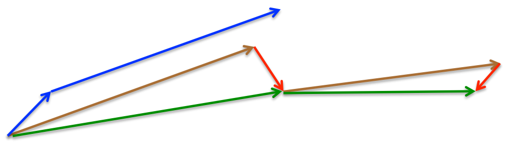
图 4: Nesterov 更新 (来源: 丁顿讲座 6c)
关于 NAG 背后的直觉，请参考这里的另一种解释，而 Ilya Sutskever 在他的博士论文 [8 中给出了更详细的概述。
既然我们能够根据错误函数的斜率调整我们的更新，并反过来加快 SGD, 我们还希望根据每个参数的重要性调整我们的更新，以执行更大或更小的更新。

Adagrad

Adagrad [9] 是一种基于梯度的优化算法，它可以做到这一点: 它根据参数调整学习率，执行较小的更新
与频繁出现的特征相关的参数 (即低学习率)，与不频繁特征相关的参数的更大更新 (即高学习率)。因此，它非常适合处理稀疏数据。Dean 等人发现，Adagrad 极大地提高了 SGD 的健壮性，并将其用于 Google 的大规模神经网络训练。在 Youtube 视频中，它学会了识别猫。此外，Pennington 等人 [11] 使用 Adagrad 来训练手套词嵌入，因为不常见的词比频繁的词需要更大的更新。
Previously, we performed an update for all parameters θθ at once as every parameter θiθiused the same learning rate ηη. As Adagrad uses a different learning rate for every parameter θiθi at every time step tt, we first show Adagrad’s per-parameter update, which we then vectorize. For brevity, we use gtgt to denote the gradient at time step tt. gt,igt,i is then the partial derivative of the objective function w.r.t. to the parameter θiθi at time step tt:
gt,i=∇θJ(θt,i)gt,i=∇θJ(θt,i).
The SGD update for every parameter θiθi at each time step tt then becomes:
θt+1,i=θt,i−η⋅gt,iθt+1,i=θt,i−η⋅gt,i.
In its update rule, Adagrad modifies the general learning rate ηη at each time step tt for every parameter θiθi based on the past gradients that have been computed for θiθi:
θt+1,i=θt,i−η√Gt,ii+ϵ⋅gt,iθt+1,i=θt,i−ηGt,ii+ϵ⋅gt,i.
Gt∈Rd×dGt∈Rd×d here is a diagonal matrix where each diagonal element i,ii,i is the sum of the squares of the gradients w.r.t. θiθi up to time step tt [12], while ϵϵ is a smoothing term that avoids division by zero (usually on the order of 1e−81e−8). Interestingly, without the square root operation, the algorithm performs much worse.
As GtGt contains the sum of the squares of the past gradients w.r.t. to all parameters θθalong its diagonal, we can now vectorize our implementation by performing a matrix-vector product ⊙⊙ between GtGt and gtgt:
θt+1=θt−η√Gt+ϵ⊙gtθt+1=θt−ηGt+ϵ⊙gt.
Adagrad 的一个主要好处是，它不需要手动调整学习率。大多数实现使用默认值 0.01，并将其保留在该值。
Adagrad 的主要缺点是它在分母中累积了平方梯度: 由于每个附加项都是正的，所以在训练过程中累积的和会不断增长。这反过来又导致学习率下降，最终变得非常小，此时算法不再能够获得额外的知识。以下算法旨在解决此缺陷。

阿德达塔

Adadelta [13] 是 Adagrad 的延伸，旨在降低其积极的、单调下降的学习率。Adadelta 没有累积所有过去的平方梯度，而是将累积过去梯度的窗口限制在某个固定大小的 ww。
梯度和不是低效地存储 ww 以前的平方梯度，而是递归地定义为所有过去平方梯度的衰减平均值。然后，时间步长 tt 上的运行平均值 E [g2] tE [g2] t 仅取决于先前的平均值和当前梯度 (与动量项相似):
E[g2]t=γE[g2]t−1+(1−γ)g2tE[g2]t=γE[g2]t−1+(1−γ)gt2.
We set γγ to a similar value as the momentum term, around 0.9. For clarity, we now rewrite our vanilla SGD update in terms of the parameter update vector ΔθtΔθt:
Δθt=−η⋅gt,iθt+1=θt+ΔθtΔθt=−η⋅gt,iθt+1=θt+Δθt
The parameter update vector of Adagrad that we derived previously thus takes the form:
Δθt=−η√Gt+ϵ⊙gtΔθt=−ηGt+ϵ⊙gt.
We now simply replace the diagonal matrix GtGt with the decaying average over past squared gradients E[g2]tE[g2]t:
Δθt=−η√E[g2]t+ϵgtΔθt=−ηE[g2]t+ϵgt.
As the denominator is just the root mean squared (RMS) error criterion of the gradient, we can replace it with the criterion short-hand:
Δθt=−ηRMS[g]tgtΔθt=−ηRMS[g]tgt.
The authors note that the units in this update (as well as in SGD, Momentum, or Adagrad) do not match, i.e. the update should have the same hypothetical units as the parameter. To realize this, they first define another exponentially decaying average, this time not of squared gradients but of squared parameter updates:
E[Δθ2]t=γE[Δθ2]t−1+(1−γ)Δθ2tE[Δθ2]t=γE[Δθ2]t−1+(1−γ)Δθt2.
The root mean squared error of parameter updates is thus:
RMS[Δθ]t=√E[Δθ2]t+ϵRMS[Δθ]t=E[Δθ2]t+ϵ.
Since RMS[Δθ]tRMS[Δθ]t is unknown, we approximate it with the RMS of parameter updates until the previous time step. Replacing the learning rate ηη in the previous update rule with RMS[Δθ]t−1RMS[Δθ]t−1 finally yields the Adadelta update rule:
Δθt=−RMS[Δθ]t−1RMS[g]tgtθt+1=θt+ΔθtΔθt=−RMS[Δθ]t−1RMS[g]tgtθt+1=θt+Δθt
With Adadelta, we do not even need to set a default learning rate, as it has been eliminated from the update rule.

RMSprop

RMSprop 是 Geoff Hinton 在 Coursera 课程第 6e 讲中提出的一种未发表的自适应学习率方法。
RMSprop 和 Adadelta 都是在大约同一时间独立开发的，这是因为需要解决 Adagrad 急剧下降的学习率。事实上，RMSprop 与我们上面导出的 Adadelta 的第一个更新向量相同:
E[g2]t=0.9E[g2]t−1+0.1g2tθt+1=θt−η√E[g2]t+ϵgtE[g2]t=0.9E[g2]t−1+0.1gt2θt+1=θt−ηE[g2]t+ϵgt
RMSprop as well divides the learning rate by an exponentially decaying average of squared gradients. Hinton suggests γγ to be set to 0.9, while a good default value for the learning rate ηη is 0.001.

Adam

自适应矩估计 (Adam) [14] 是计算每个参数自适应学习率的另一种方法。除了存储像 Adadelta 和 RMSprop 这样的过去平方梯度 vtvt 的指数衰减平均值之外，Adam 还保持过去梯度 mtmt 的指数衰减平均值，类似于动量。虽然动量可以被视为沿着斜坡运行的球，但亚当的行为就像一个带有摩擦的重球，因此在误差面 [15 中更喜欢平坦的最小值。我们分别计算过去和过去平方梯度 mtmt 和 vtvt 的衰减平均值，如下所示:
mt=β1mt−1+(1−β1)gtvt=β2vt−1+(1−β2)g2tmt=β1mt−1+(1−β1)gtvt=β2vt−1+(1−β2)gt2
mtmt and vtvt are estimates of the first moment (the mean) and the second moment (the uncentered variance) of the gradients respectively, hence the name of the method. As mtmt and vtvt are initialized as vectors of 0’s, the authors of Adam observe that they are biased towards zero, especially during the initial time steps, and especially when the decay rates are small (i.e. β1β1 and β2β2 are close to 1).
They counteract these biases by computing bias-corrected first and second moment estimates:
^mt=mt1−βt1^vt=vt1−βt2m^t=mt1−β1tv^t=vt1−β2t
They then use these to update the parameters just as we have seen in Adadelta and RMSprop, which yields the Adam update rule:
θt+1=θt−η√^vt+ϵ^mtθt+1=θt−ηv^t+ϵm^t.
The authors propose default values of 0.9 for β1β1, 0.999 for β2β2, and 10−810−8 for ϵϵ. They show empirically that Adam works well in practice and compares favorably to other adaptive learning-method algorithms.

AdaMax

The vtvt factor in the Adam update rule scales the gradient inversely proportionally to the ℓ2ℓ2 norm of the past gradients (via the vt−1vt−1 term) and current gradient |gt|2|gt|2:
vt=β2vt−1+(1−β2)|gt|2vt=β2vt−1+(1−β2)|gt|2
We can generalize this update to the ℓpℓp norm. Note that Kingma and Ba also parameterize β2β2 as βp2β2p:
vt=βp2vt−1+(1−βp2)|gt|pvt=β2pvt−1+(1−β2p)|gt|p
Norms for large pp values generally become numerically unstable, which is why ℓ1ℓ1 and ℓ2ℓ2 norms are most common in practice. However, ℓ∞ℓ∞ also generally exhibits stable behavior. For this reason, the authors propose AdaMax (Kingma and Ba, 2015) and show that vtvt with ℓ∞ℓ∞ converges to the following more stable value. To avoid confusion with Adam, we use utut to denote the infinity norm-constrained vtvt:
ut=β∞2vt−1+(1−β∞2)|gt|∞=max(β2⋅vt−1,|gt|)ut=β2∞vt−1+(1−β2∞)|gt|∞=max(β2⋅vt−1,|gt|)
We can now plug this into the Adam update equation by replacing √^vt+ϵv^t+ϵ with utut to obtain the AdaMax update rule:
θt+1=θt−ηut^mtθt+1=θt−ηutm^t
Note that as utut relies on the maxmax operation, it is not as suggestible to bias towards zero as mtmt and vtvt in Adam, which is why we do not need to compute a bias correction for utut. Good default values are again η=0.002η=0.002, β1=0.9β1=0.9, and β2=0.999β2=0.999.

Nadam

正如我们以前所看到的，亚当可以被视为 RMSprop 和动量的组合: RMSprop 贡献了过去平方梯度 vtvt 的指数衰减平均值, 虽然动量占过去梯度 mtmt 的指数衰减平均值我们也看到了 Nesterov 加速梯度 (NAG) 优于香草动量。
因此，Nadam (Nesterov 加速自适应矩估计) [16] 将 Adam 和 NAG 结合在了一起。为了将 NAG 合并到 Adam 中，我们需要修改它的动量项 mtmt。
首先，让我们回顾一下使用我们当前符号的动量更新规则:
gt=∇θtJ(θt)mt=γmt−1+ηgtθt+1=θt−mtgt=∇θtJ(θt)mt=γmt−1+ηgtθt+1=θt−mt
where JJ is our objective function, γγ is the momentum decay term, and ηη is our step size. Expanding the third equation above yields:
θt+1=θt−(γmt−1+ηgt)θt+1=θt−(γmt−1+ηgt)
This demonstrates again that momentum involves taking a step in the direction of the previous momentum vector and a step in the direction of the current gradient.
NAG then allows us to perform a more accurate step in the gradient direction by updating the parameters with the momentum step before computing the gradient. We thus only need to modify the gradient gtgt to arrive at NAG:
gt=∇θtJ(θt−γmt−1)mt=γmt−1+ηgtθt+1=θt−mtgt=∇θtJ(θt−γmt−1)mt=γmt−1+ηgtθt+1=θt−mt
Dozat proposes to modify NAG the following way: Rather than applying the momentum step twice — one time for updating the gradient gtgt and a second time for updating the parameters θt+1θt+1 — we now apply the look-ahead momentum vector directly to update the current parameters:
gt=∇θtJ(θt)mt=γmt−1+ηgtθt+1=θt−(γmt+ηgt)gt=∇θtJ(θt)mt=γmt−1+ηgtθt+1=θt−(γmt+ηgt)
Notice that rather than utilizing the previous momentum vector mt−1mt−1 as in the equation of the expanded momentum update rule above, we now use the current momentum vector mtmt to look ahead. In order to add Nesterov momentum to Adam, we can thus similarly replace the previous momentum vector with the current momentum vector. First, recall that the Adam update rule is the following (note that we do not need to modify ^vtv^t):
mt=β1mt−1+(1−β1)gt^mt=mt1−βt1θt+1=θt−η√^vt+ϵ^mtmt=β1mt−1+(1−β1)gtm^t=mt1−β1tθt+1=θt−ηv^t+ϵm^t
Expanding the second equation with the definitions of ^mtm^t and mtmt in turn gives us:
θt+1=θt−η√^vt+ϵ(β1mt−11−βt1+(1−β1)gt1−βt1)θt+1=θt−ηv^t+ϵ(β1mt−11−β1t+(1−β1)gt1−β1t)
Note that β1mt−11−βt1β1mt−11−β1t is just the bias-corrected estimate of the momentum vector of the previous time step. We can thus replace it with ^mt−1m^t−1:
θt+1=θt−η√^vt+ϵ(β1^mt−1+(1−β1)gt1−βt1)θt+1=θt−ηv^t+ϵ(β1m^t−1+(1−β1)gt1−β1t)
Note that for simplicity, we ignore that the denominator is 1−βt11−β1t and not 1−βt−111−β1t−1 as we will replace the denominator in the next step anyway. This equation again looks very similar to our expanded momentum update rule above. We can now add Nesterov momentum just as we did previously by simply replacing this bias-corrected estimate of the momentum vector of the previous time step ^mt−1m^t−1 with the bias-corrected estimate of the current momentum vector ^mtm^t, which gives us the Nadam update rule:
θt+1=θt−η√^vt+ϵ(β1^mt+(1−β1)gt1−βt1)θt+1=θt−ηv^t+ϵ(β1m^t+(1−β1)gt1−β1t)

AMSGrad

由于自适应学习率方法已经成为训练神经网络的标准，在某些情况下, 例如，对于物体识别 [17] 或机器翻译 [18]，它们未能收敛到最优解，并且被具有动量的 SGD 超越。
Reddi 等人 (2018) [19] 正式提出了这个问题，并指出过去平方梯度的指数移动平均值是自适应学习率方法泛化性能差的原因。回想一下，指数平均的引入是有充分动机的: 随着训练的进行，学习率应该会变得非常小，这是 Adagrad 算法的关键缺陷。然而，梯度的这种短期记忆在其他情况下成为障碍。
在 Adam 收敛到次优解的设置中，已经观察到一些小批量提供了大量的信息梯度，但是由于这些小批量很少发生，指数平均减少了它们的影响, 这导致了收敛不良。作者为一个简单的凸优化问题提供了一个例子，在这个问题中，Adam 可以观察到相同的行为。
To fix this behaviour, the authors propose a new algorithm, AMSGrad that uses the maximum of past squared gradients vtvt rather than the exponential average to update the parameters. vtvt is defined the same as in Adam above:
vt=β2vt−1+(1−β2)g2tvt=β2vt−1+(1−β2)gt2
Instead of using vtvt (or its bias-corrected version ^vtv^t) directly, we now employ the previous vt−1vt−1 if it is larger than the current one:
^vt=max(^vt−1,vt)v^t=max(v^t−1,vt)
This way, AMSGrad results in a non-increasing step size, which avoids the problems suffered by Adam. For simplicity, the authors also remove the debiasing step that we have seen in Adam. The full AMSGrad update without bias-corrected estimates can be seen below:
mt=β1mt−1+(1−β1)gtvt=β2vt−1+(1−β2)g2t^vt=max(^vt−1,vt)θt+1=θt−η√^vt+ϵmtmt=β1mt−1+(1−β1)gtvt=β2vt−1+(1−β2)gt2v^t=max(v^t−1,vt)θt+1=θt−ηv^t+ϵmt
作者观察到，与 Adam 相比，在小数据集和 CIFAR-10 上的性能有所提高。然而，其他实验显示出与 Adam 相似或更差的性能。AMSGrad 是否能够在实践中始终超越亚当还有待观察。有关深度学习优化的最新进展的更多信息，请参阅此博客文章。

算法可视化

以下两个动画 (图像信用: Alec Radford) 为大多数所提出的优化方法的优化行为提供了一些直观的信息。这里还可以查看 Karpathy 对同一图像的描述，以及所讨论算法的另一个简明概述。
在图 5 中，我们看到随着时间的推移，它们在损失表面轮廓 (Beale 函数) 上的行为。请注意，Adagrad 、 Adadelta 和 RMSprop 几乎立即朝着正确的方向出发，并以同样的速度收敛，而动量和 NAG 则偏离了轨道, 让人想起一个滚下山坡的球。然而，NAG 很快就能纠正它的路线，因为它通过向前看并走向最低限度来提高响应能力。
图 6 显示了算法在鞍点的行为，即一个维度具有正斜率，而另一个维度具有负斜率的点, 正如我们之前提到的，这给 SGD 带来了困难。请注意，SGD 、 Momentum 和 NAG 发现很难打破对称，尽管后两者最终设法逃离鞍点，而 Adagrad 、 RMSprop 、 adadelta 很快就沿着负斜坡往下走。

Image 5: SGD optimization on loss surface contours	Image 6: SGD optimization on saddle point

正如我们所看到的，自适应学习率方法，即 Adagrad 、 Adadelta 、 RMSprop 和 Adam 最合适，为这些场景提供了最佳的收敛。
注意: 如果你对可视化这些或其他优化算法感兴趣，请参考这个有用的教程。

使用哪个优化器？

那么，你现在应该使用哪个优化器？如果你的输入数据是稀疏的，那么你可能会使用一种自适应学习率方法来获得最好的结果。另一个好处是，你不需要调整学习率，但是使用默认值可能会获得最佳效果。
总之，RMSprop 是 Adagrad 的一个扩展，它处理的是其学习率急剧下降的问题。它与 Adadelta 相同，只是 Adadelta 在 numinator 更新规则中使用了参数更新的 RMS。最后，Adam 为 RMSprop 增加了偏差修正和动量。在这方面，RMSprop 、 Adadelta 和 Adam 是非常相似的算法，在类似的情况下表现良好。Kingma 等人 [14: 1] 表明，随着梯度变得稀疏，其偏差校正有助于 Adam 在优化结束时稍微优于 RMSprop。在这方面，亚当可能是最好的选择。
有趣的是，最近的许多论文使用了没有动量的香草 SGD 和简单的学习率退火时间表。如前所述，SGD 通常能够找到最小值，但是它可能比一些优化器需要更长的时间，更依赖于稳健的初始化和退火时间表, 可能会陷入鞍点，而不是局部最小值。因此，如果你关心快速收敛并训练深度或复杂的神经网络，你应该选择一种自适应学习率方法。

SGD 的并行化和分发

鉴于大规模数据解决方案的普遍存在和低商品集群的可用性，分发 SGD 以进一步加快速度是一个明显的选择。
SGD 本身具有内在的顺序性: 一步一步地，我们朝着最小目标前进。运行它提供了良好的收敛，但在大型数据集上可能会特别慢。相比之下，异步运行 SGD 更快，但是工人之间的通信不理想会导致收敛不良。此外，我们还可以在一台机器上并行 SGD，而不需要大型计算集群。以下是为优化并行和分布式 SGD 而提出的算法和体系结构。

Hogwild!

牛等人 [20] 介绍了一个名为 Hogwild 的更新方案!允许在 cpu 上并行执行 SGD 更新。允许处理器在不锁定参数的情况下访问共享内存。只有当输入数据稀疏时，这才有效，因为每次更新只会修改所有参数的一小部分。他们表明，在这种情况下，更新方案几乎达到了最佳的收敛速度，因为处理器不太可能覆盖有用的信息。

Downpour SGD

倾盆大雨 SGD 是 SGD 的异步变体，由 Dean 等人在 Google 的 DistBelief 框架 (TensorFlow 的前身) 中使用。它在训练数据的子集上并行运行模型的多个副本。这些模型将它们的更新发送到参数服务器，该服务器在许多机器上被分割。每台机器负责存储和更新模型参数的一小部分。然而，由于副本之间不会通过共享权重或更新等方式进行通信，因此它们的参数不断有发散的风险，阻碍了收敛。

Delay-tolerant Algorithms for SGD

McMahan 和 Streeter [21] 通过开发不仅适应过去梯度，而且适应更新延迟的延迟容忍算法，将 AdaGrad 扩展到并行设置。这在实践中被证明是有效的。

TensorFlow

TensorFlow [22] 是 Google 最近为大规模机器学习模型的实现和部署而开发的开源框架。它是基于他们在 DistBelief 上的经验，已经在内部用于在大型移动设备和大型分布式系统上执行计算。对于分布式执行，计算图被分成每个设备的子图，并使用发送/接收节点对进行通信。然而，TensorFlow 的开源版本目前不支持分布式功能 (请参见此处)。
更新 13.04.16: TensorFlow 的分布式版本已经发布。

Elastic Averaging SGD

Zhang 等人 [23] 提出了弹性平均 SGD (EASGD)，它将异步 SGD 工人的参数与弹性力联系起来，即参数服务器存储的中心变量。这使得局部变量可以与中心变量进一步波动，这在理论上允许对参数空间进行更多的探索。他们经验表明，这种勘探能力的增加通过找到新的局部最优来提高性能。

Additional strategies for optimizing SGD

最后，我们引入了额外的策略，这些策略可以与前面提到的任何算法一起使用，以进一步提高 SGD 的性能。有关其他一些常见技巧的概述，请参考 [24]。

Shuffling and Curriculum Learning

通常，我们希望避免以有意义的顺序向我们的模型提供训练示例，因为这可能会偏向优化算法。因此，在每个时代之后洗牌训练数据通常是一个好主意。
另一方面，对于一些我们旨在逐步解决更棘手问题的情况，以有意义的顺序提供培训示例实际上可能会提高性能和更好的收敛。建立这种有意义秩序的方法叫做课程学习 [25]。
Zaremba 和 Sutskever [26] 只能训练 LSTMs 使用课程学习来评估简单的项目，并表明组合或混合策略比天真的策略更好, 通过增加难度对例子进行排序。

Batch normalization

为了便于学习，我们通常通过用零均值和单位方差初始化参数来标准化参数的初始值。随着训练的进行，我们对参数进行了不同程度的更新，我们失去了这种标准化，这减缓了训练速度，并随着网络的深入而放大了变化。
批标准化 [27] 为每个迷你批重新建立这些标准化，并且更改也会通过操作反向传播。通过将标准化作为模型架构的一部分，我们能够使用更高的学习率，并且对初始化参数的关注更少。批标准化还充当了监管机构的角色，减少 (有时甚至消除) 辍学的需求。

Early stopping

据 Geoff Hinton 说: “提前停止 (是) 美丽的免费午餐” (NIPS 2015 教程幻灯片，幻灯片 63)。因此，您应该始终在培训期间监控验证集的错误，如果验证错误没有得到足够的改进，则停止 (耐心等待)。

Gradient noise

Neelakantan et al. [28] add noise that follows a Gaussian distribution N(0,σ2t)N(0,σt2) to each gradient update:
gt,i=gt,i+N(0,σ2t)gt,i=gt,i+N(0,σt2).
They anneal the variance according to the following schedule:
σ2t=η(1+t)γσt2=η(1+t)γ.
他们表明，增加这种噪声使得网络对糟糕的初始化更加健壮，并有助于训练特别深入和复杂的网络。他们怀疑，增加的噪音给了模型更多的机会逃避和发现新的局部最小值，这对于更深入的模型来说更常见。

Conclusion

在这篇博文中，我们初步研究了梯度下降的三种变体，其中最受欢迎的是小批量梯度下降。然后，我们研究了优化 SGD 最常用的算法: 动量、 Nesterov 加速梯度、 Adagrad 、 Adadelta 、 RMSprop 、 Adam，以及优化异步 SGD最后，我们考虑了其他改进 SGD 的策略，如洗牌和课程学习、批量标准化和提前停止。
我希望这篇博客文章能够为你提供一些对不同优化算法的动机和行为的直觉。我错过了哪些明显的算法来改进 SGD？你自己用什么技巧来促进 SGD 的培训？在下面的评论中告诉我。

Acknowledgements

Thanks to Denny Britz and Cesar Salgado for reading drafts of this post and providing suggestions.

Printable version and citation

This blog post is also available as an article on arXiv, in case you want to refer to it later.
In case you found it helpful, consider citing the corresponding arXiv article as:
Sebastian Ruder (2016). An overview of gradient descent optimisation algorithms. arXiv preprint arXiv:1609.04747.

Translations

This blog post has been translated into the following languages:

• Japanese
• Chinese
• Korean

Image credit for cover photo: Karpathy’s beautiful loss functions tumblr

1. H. Robinds and S. Monro, “A stochastic approximation method,” Annals of Mathematical Statistics, vol. 22, pp. 400–407, 1951. ↩︎
   
2. Darken, C., Chang, J., & Moody, J. (1992). Learning rate schedules for faster stochastic gradient search. Neural Networks for Signal Processing II Proceedings of the 1992 IEEE Workshop, (September), 1–11. http://doi.org/10.1109/NNSP.1992.253713 ↩︎
   
3. Dauphin, Y., Pascanu, R., Gulcehre, C., Cho, K., Ganguli, S., & Bengio, Y. (2014). Identifying and attacking the saddle point problem in high-dimensional non-convex optimization. arXiv, 1–14. Retrieved from http://arxiv.org/abs/1406.2572 ↩︎
   
4. Sutton, R. S. (1986). Two problems with backpropagation and other steepest-descent learning procedures for networks. Proc. 8th Annual Conf. Cognitive Science Society. ↩︎
   
5. Qian, N. (1999). On the momentum term in gradient descent learning algorithms. Neural Networks : The Official Journal of the International Neural Network Society, 12(1), 145–151. http://doi.org/10.1016/S0893-6080(98)00116-600116-6) ↩︎
   
6. Nesterov, Y. (1983). A method for unconstrained convex minimization problem with the rate of convergence o(1/k2). Doklady ANSSSR (translated as Soviet.Math.Docl.), vol. 269, pp. 543– 547. ↩︎
   
7. Bengio, Y., Boulanger-Lewandowski, N., & Pascanu, R. (2012). Advances in Optimizing Recurrent Networks. Retrieved from http://arxiv.org/abs/1212.0901 ↩︎
   
8. Sutskever, I. (2013). Training Recurrent neural Networks. PhD Thesis. ↩︎
   
9. Duchi, J., Hazan, E., & Singer, Y. (2011). Adaptive Subgradient Methods for Online Learning and Stochastic Optimization. Journal of Machine Learning Research, 12, 2121–2159. Retrieved from http://jmlr.org/papers/v12/duchi11a.html ↩︎
   
10. Dean, J., Corrado, G. S., Monga, R., Chen, K., Devin, M., Le, Q. V, … Ng, A. Y. (2012). Large Scale Distributed Deep Networks. NIPS 2012: Neural Information Processing Systems, 1–11. http://papers.nips.cc/paper/4687-large-scale-distributed-deep-networks.pdf ↩︎ ↩︎
    
11. Pennington, J., Socher, R., & Manning, C. D. (2014). Glove: Global Vectors for Word Representation. Proceedings of the 2014 Conference on Empirical Methods in Natural Language Processing, 1532–1543. http://doi.org/10.3115/v1/D14-1162 ↩︎
    
12. Duchi et al. [3] give this matrix as an alternative to the full matrix containing the outer products of all previous gradients, as the computation of the matrix square root is infeasible even for a moderate number of parameters dd. ↩︎
    
13. Zeiler, M. D. (2012). ADADELTA: An Adaptive Learning Rate Method. Retrieved from http://arxiv.org/abs/1212.5701 ↩︎
    
14. Kingma, D. P., & Ba, J. L. (2015). Adam: a Method for Stochastic Optimization. International Conference on Learning Representations, 1–13. ↩︎ ↩︎
    
15. Heusel, M., Ramsauer, H., Unterthiner, T., Nessler, B., & Hochreiter, S. (2017). GANs Trained by a Two Time-Scale Update Rule Converge to a Local Nash Equilibrium. In Advances in Neural Information Processing Systems 30 (NIPS 2017). ↩︎
    
16. Dozat, T. (2016). Incorporating Nesterov Momentum into Adam. ICLR Workshop, (1), 2013–2016. ↩︎
    
17. Huang, G., Liu, Z., Weinberger, K. Q., & van der Maaten, L. (2017). Densely Connected Convolutional Networks. In Proceedings of CVPR 2017. ↩︎
    
18. Johnson, M., Schuster, M., Le, Q. V, Krikun, M., Wu, Y., Chen, Z., … Dean, J. (2016). Google’s Multilingual Neural Machine Translation System: Enabling Zero-Shot Translation. arXiv Preprint arXiv:1611.0455. ↩︎
    
19. Reddi, Sashank J., Kale, Satyen, & Kumar, Sanjiv. On the Convergence of Adam and Beyond. Proceedings of ICLR 2018. ↩︎
    
20. Niu, F., Recht, B., Christopher, R., & Wright, S. J. (2011). Hogwild! : A Lock-Free Approach to Parallelizing Stochastic Gradient Descent, 1–22. ↩︎
    
21. Mcmahan, H. B., & Streeter, M. (2014). Delay-Tolerant Algorithms for Asynchronous Distributed Online Learning. Advances in Neural Information Processing Systems (Proceedings of NIPS), 1–9. Retrieved from http://papers.nips.cc/paper/5242-delay-tolerant-algorithms-for-asynchronous-distributed-online-learning.pdf ↩︎
    
22. Abadi, M., Agarwal, A., Barham, P., Brevdo, E., Chen, Z., Citro, C., … Zheng, X. (2015). TensorFlow : Large-Scale Machine Learning on Heterogeneous Distributed Systems. ↩︎
    
23. Zhang, S., Choromanska, A., & LeCun, Y. (2015). Deep learning with Elastic Averaging SGD. Neural Information Processing Systems Conference (NIPS 2015), 1–24. Retrieved from http://arxiv.org/abs/1412.6651 ↩︎
    
24. LeCun, Y., Bottou, L., Orr, G. B., & Müller, K. R. (1998). Efficient BackProp. Neural Networks: Tricks of the Trade, 1524, 9–50. http://doi.org/10.1007/3-540-49430-8_2 ↩︎
    
25. Bengio, Y., Louradour, J., Collobert, R., & Weston, J. (2009). Curriculum learning. Proceedings of the 26th Annual International Conference on Machine Learning, 41–48. http://doi.org/10.1145/1553374.1553380 ↩︎
    
26. Zaremba, W., & Sutskever, I. (2014). Learning to Execute, 1–25. Retrieved from http://arxiv.org/abs/1410.4615 ↩︎
    
27. Ioffe, S., & Szegedy, C. (2015). Batch Normalization : Accelerating Deep Network Training by Reducing Internal Covariate Shift. arXiv Preprint arXiv:1502.03167v3. ↩︎
    
28. Neelakantan, A., Vilnis, L., Le, Q. V., Sutskever, I., Kaiser, L., Kurach, K., & Martens, J. (2015). Adding Gradient Noise Improves Learning for Very Deep Networks, 1–11. Retrieved from http://arxiv.org/abs/1511.06807 ↩︎