相比一维数据的自己跟自己过不去，二维数据，就是自己跟其他数据过不去。

这里我们先介绍的是，二个数据间的差异。

差异检验

两组比较

• 正态分布数据, t 检验

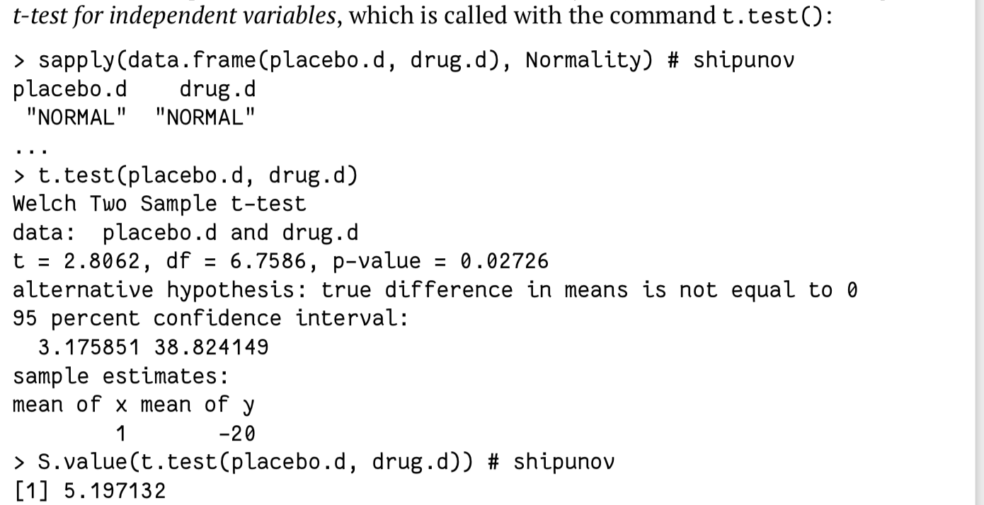
默认下使用的是Welch Two Sample t-test，不需要满足方差齐性：

> t.test(a2,a3, var.equal=T)
    Two Sample t-test
data:  a2 and a3
t = 3.746, df = 198, p-value = 0.0002356
alternative hypothesis: true difference in means is not equal to 0
95 percent confidence interval:
 1.592921 5.134473
sample estimates:
mean of x mean of y 
 34.64285  31.27916

可以修改。

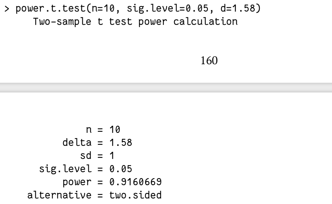
还可以通过指定信息，获得可能出现二型错误（假阴性）的可能：

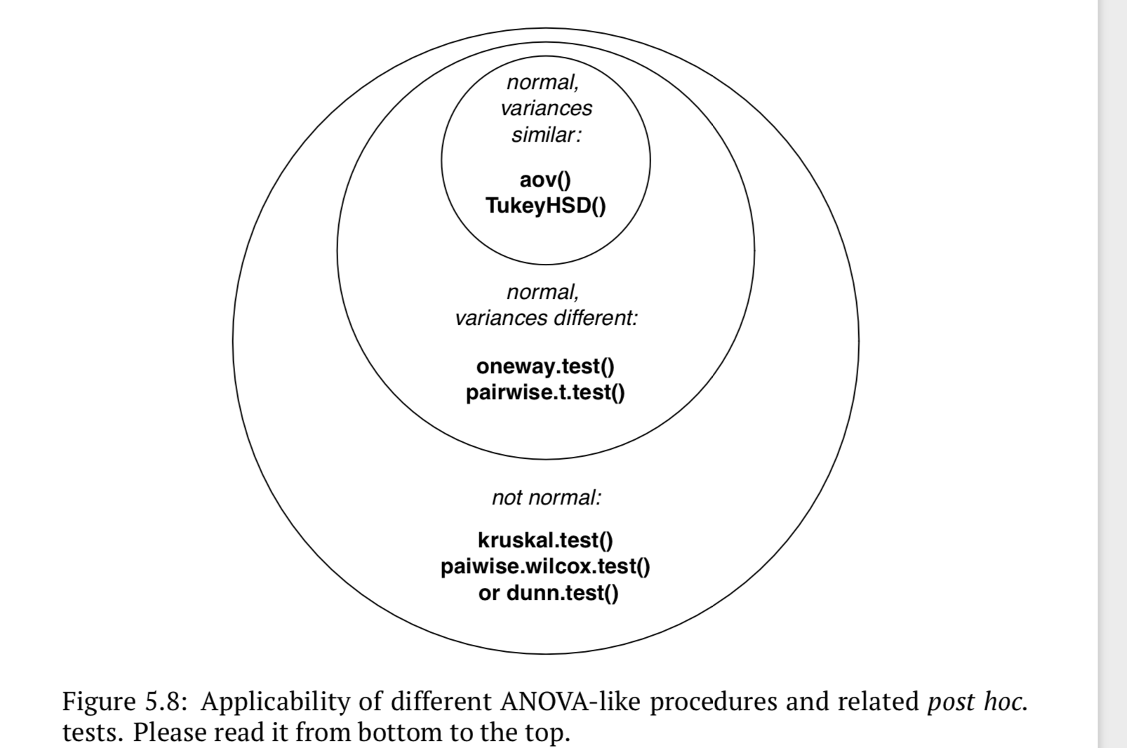
多组比较

单纯的通过多组在两两比较来实现多组比较，有以下坏处：

• 容易增大错误发生的可能性
• 繁琐且麻烦

参数检验、方差齐性

• anova(ANalysis Of VAriance)

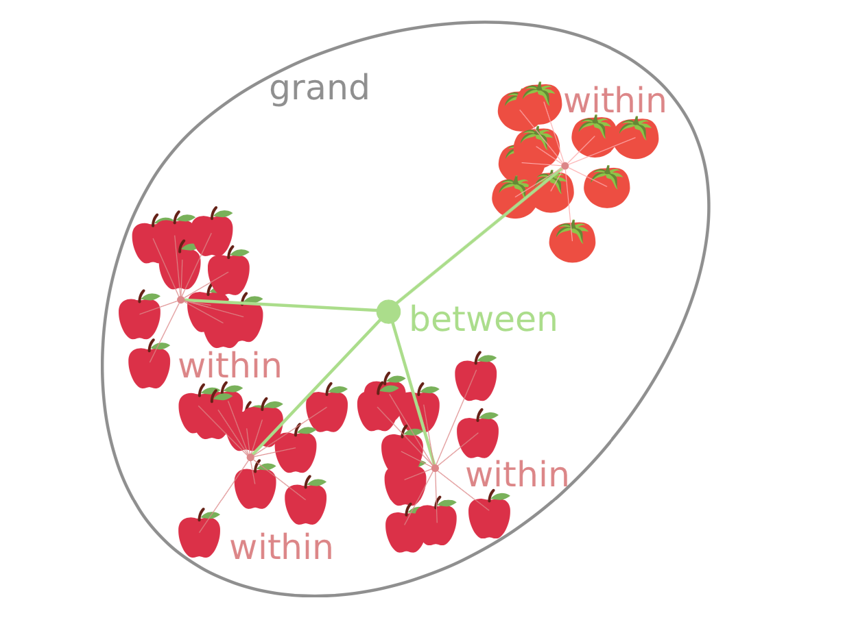
我们并不能直接通过anova 获得组别的差异信息：

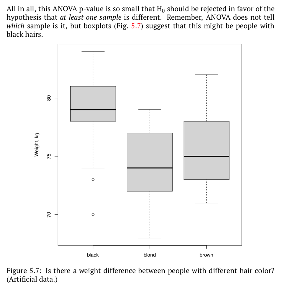
但可以通过anova 得到结果后，再通过其他检测进一步验证（比如箱线图）。

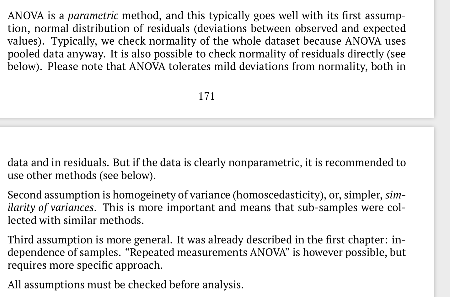
三个前提：

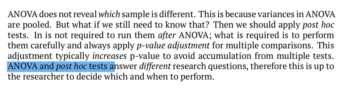
下面几个方法可以验证anova 中显著差异的分组：

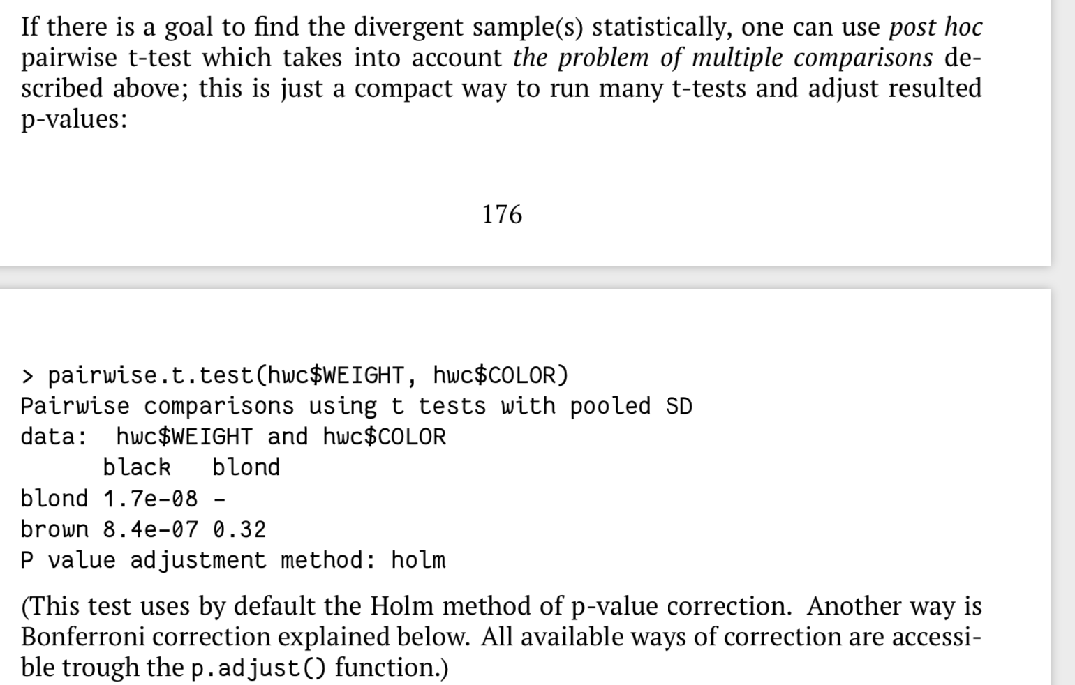
• 配对t 检验

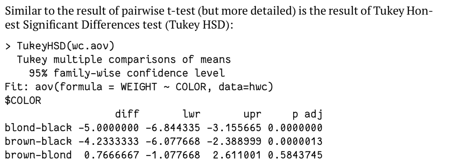
• tukey HSD test

• post hoc test

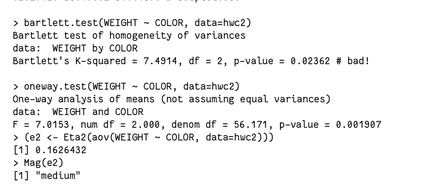
参数、方差非齐性

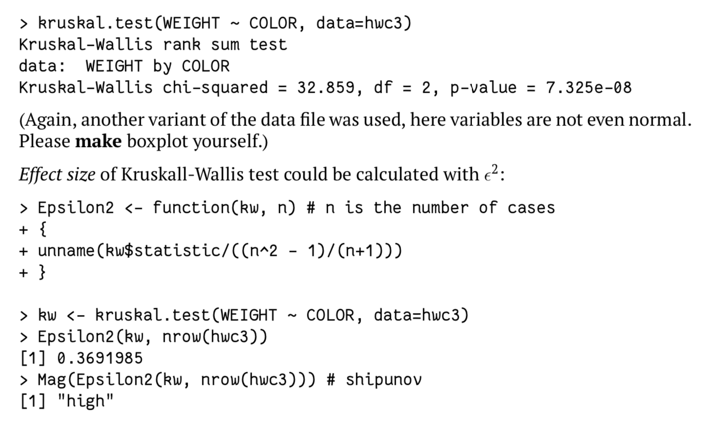
非参数方法

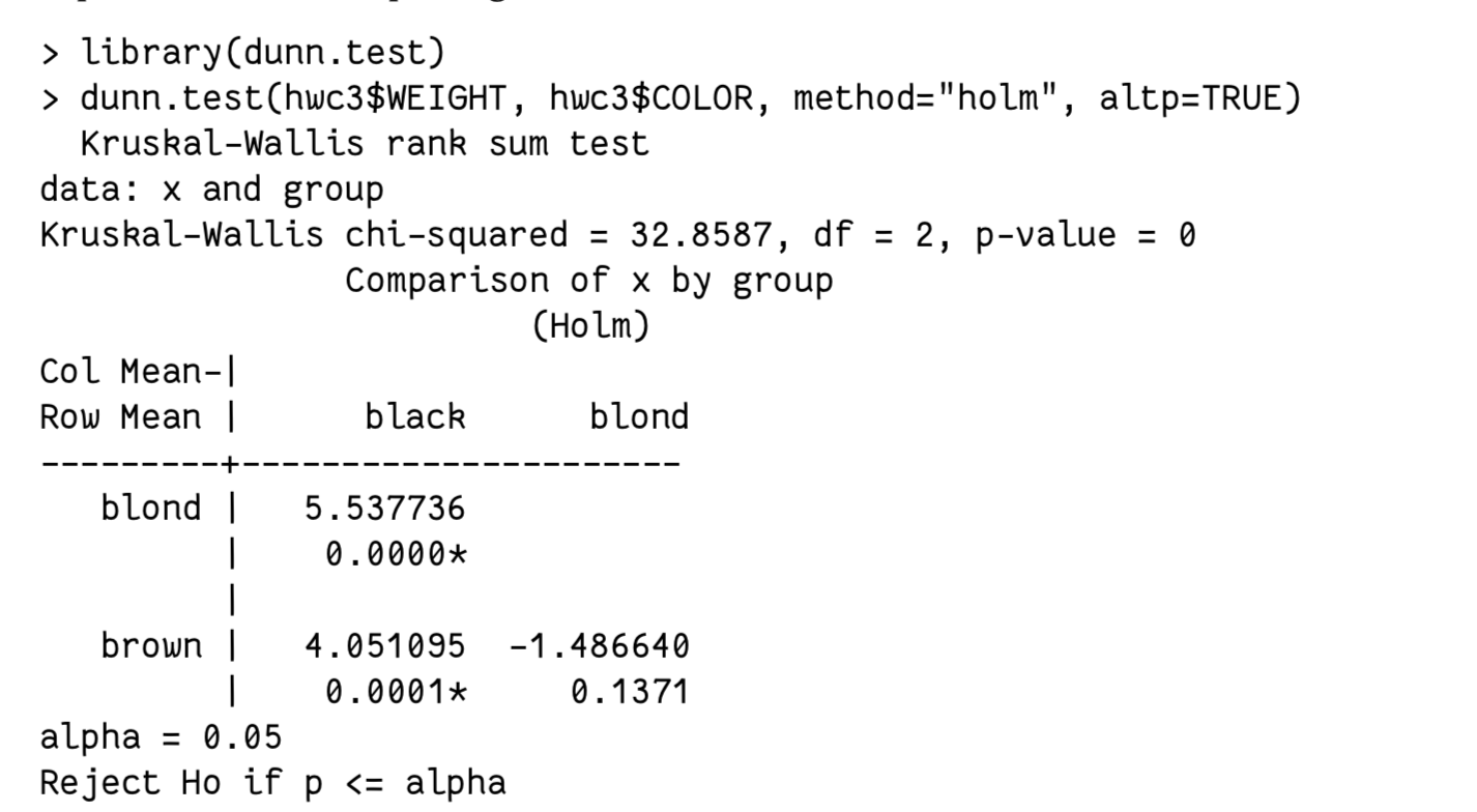
• kruskal.test

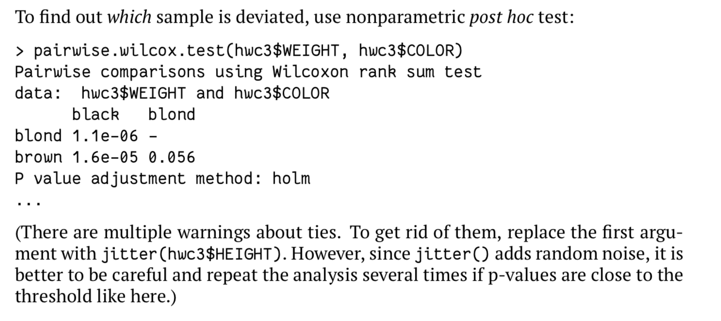
验证方法也有所不同，使用非参数的配对秩和检验：

dunn.test：

方差齐性检验

• F 检验

> var.test(a$a1, a$a2)
    F test to compare two variances
data:  a$a1 and a$a2
F = 0.21446, num df = 19, denom df = 19, p-value = 0.00153
alternative hypothesis: true ratio of variances is not equal to 1
95 percent confidence interval:
 0.08488522 0.54181849
sample estimates:
ratio of variances 
         0.2144583

• sign test

• 多组比较bartlett.test：

> bartlett.test(bb~aa, data=a1)
    Bartlett test of homogeneity of variances
data:  bb by aa
Bartlett's K-squared = 0.11603, df = 2, p-value = 0.9436

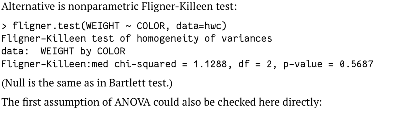
• 非参数方法Fligner-Killeen test：

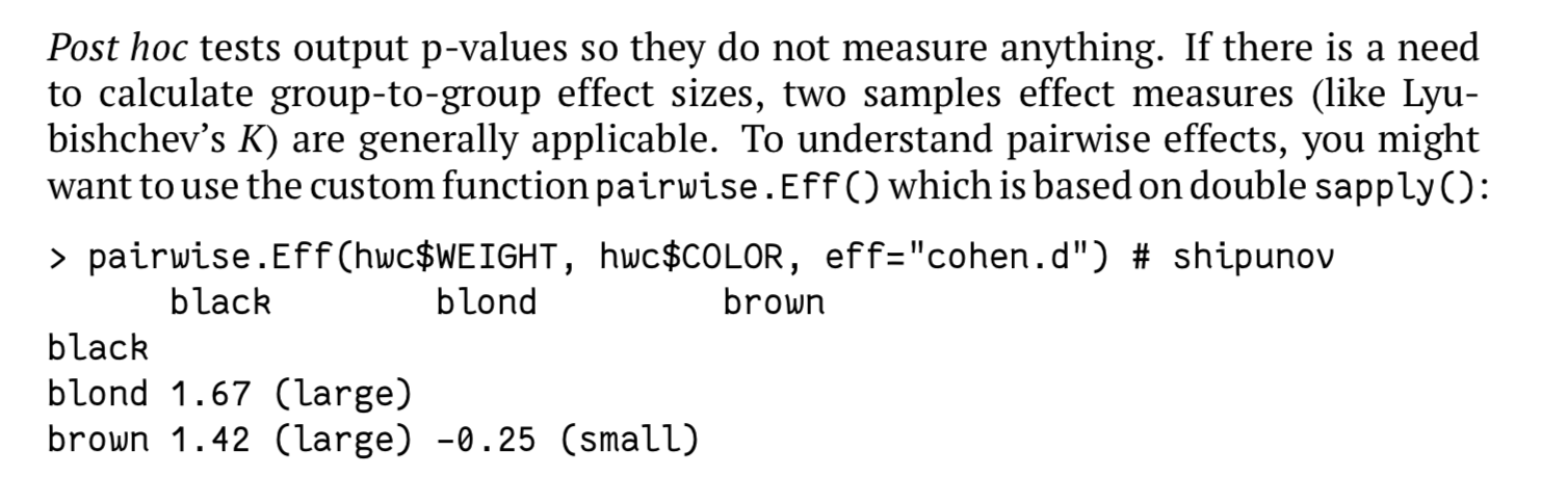
效应估计

分别对应参数模型与非参数模型：

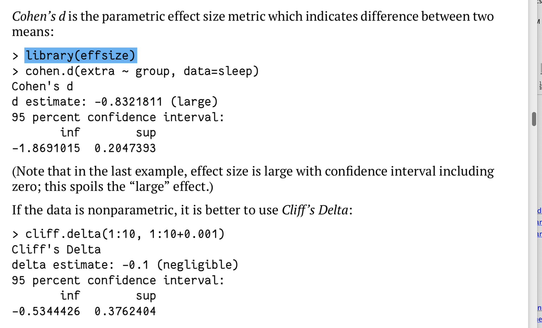
此外，还有计算差异系数的（有点类似变异系数的计算）：

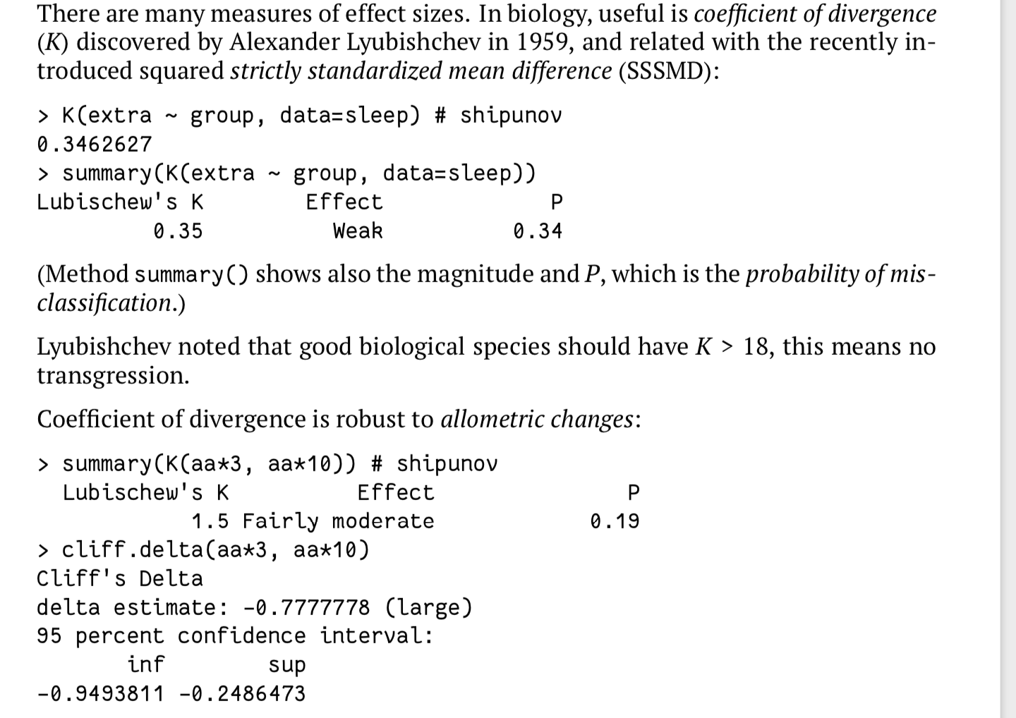
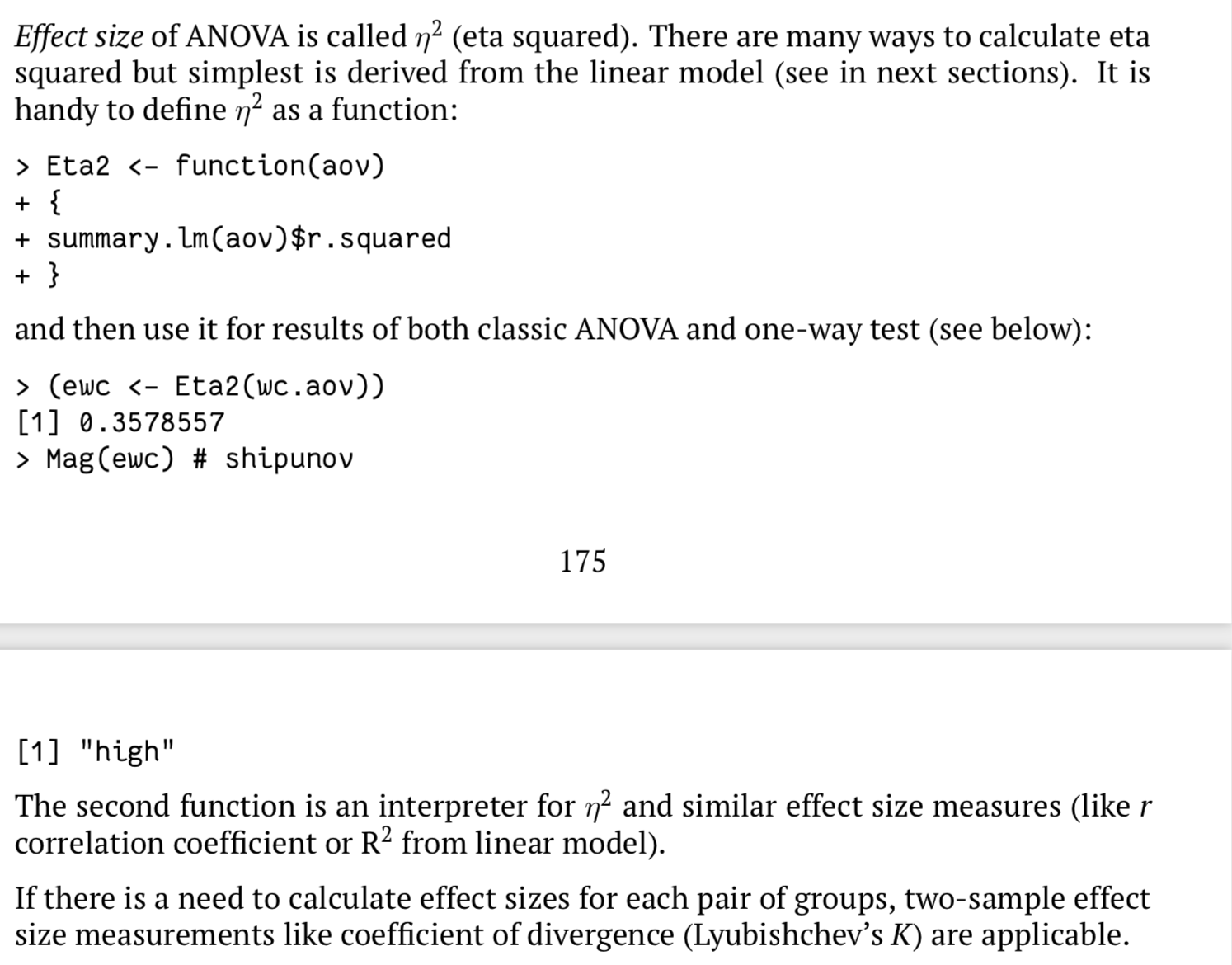
此外，还有anova 的估计方法：

总结

步骤：

• 数据结构和类型是否规范、是否有缺失值、是否有非法数据
• 箱线图绘图
• 正态性检验、方差齐性检验
• 差异检验
• 效应检验
• 具体配对检验（post hoc test）