Dynamic Filtering with Large Sampling Field for ConvNets

主要工作

这是ECCV2018的一篇文章，之所以会看他，主要是因为想要了解下dynamic filtering的处理过程，这里没有直接看当初提出这种设计的那篇文章：Dynamic Filter Networks（http://papers.nips.cc/paper/6578-dynamic-filter-networks.pdf），而是先看了下这篇，因为其中的一些总结指出了原始动态卷积的一些不足，同时也对相关的工作进行了一个简单的总结。感觉还有些用。

本文基于Dynamic Filter Network，通过更大范围采样扩大感受野，获得更有效的局部梯度，同时使用注意力机制，针对不同位置进行不同的权重处理，可以获得更为锐利有效的输出特征。

This work introduces Dynamic Filtering with Large Sampling Field (LS-DFN) to learn dynamic position-specific kernels and takes advantage of very large receptive fields and local gradients. Thanks to the large ERF in a single layer, LS-DFNs have better performance in most general tasks. With local gradients and dynamic kernels, LS-DFNs are able to produce much sharper output features, which is beneficial especially in dense prediction tasks such as optical flow estimation.

主要关键点：

• 动态滤波器网络
  • Dynamic Filter Networks [5] are originally proposed by Brabandere et al. to provide custom parameters for different input data. This architecture is powerful and more flexible since the kernels are dynamically conditioned on inputs.
  • Recently, several task-oriented objectives and extensions have been developed.
    • Deformable convolution [4] can be seen as an extension of DFNs that discovers geometric-invariant features.
    • Segmentation-aware convolution [10] explicitly takes advantage of prior segmentation information to refine feature boundaries via attention masks.
  • Different from the models mentioned above, our LS-DFNs aim at constructing large receptive fields and receiving local gradients to produce sharper and more semantic feature maps.
• 大范围采样扩大感受野
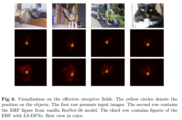
  • Wenjie et al. propose the concept of effective receptive field (ERF) and the mathematical measure using partial derivatives. The experimental results verify that the ERF usually occupies only a small fraction of the theoretical receptive field [20] which is the input region that an output unit de-pends on. Therefore, this has attracted lots of research especially in deep learning based computer vision.
    • For instance, Chen et al. [1] propose dilated convolution with hole algorithm and achieve better results on semantic segmentation.
    • Dai et al. [4] propose to dynamically learn the spatial o set of the kernels at each position so that those kernels can observe wider regions in the bottom layer with irregular shapes.
  • However, some applications such as large motion estimation and large object detection even require larger ERF.
• 残差学习
  • Generally, residual learning reduces the difficulties of directly learning the objectives by learning their residual discrepancy of an identity function.
  • ResNets [11] are proposed to learn residual features of identity mapping via short-cut connection and helps deepen CNNs to over 100 layers easily. There have been plenty of works adopting residual learning to alleviate the problem of divergence and generate richer features.
    • Kim et al. [14] adopt residual learning to model multimodal data in visual QA. Long et al. [19] learn residual transfer networks for domain adaptation.
    • Besides, Fei Wang et al. [29] apply residual learning to alleviate the problem of repeated features in attention model.
  • We apply residual learning strategy to learn residual discrepancy for identical convolutional kernels. By doing so, we can ensure valid gradients’ back-propagation so that the LS-DFNs can easily converge in real-world datasets.
• 注意力加权，区分重要性
  • For the purpose of recognizing important features in deep learning unsupervisedly, attention mechanism has been applied to lots of vision tasks including image classification [29], semantic segmentation [10], action recognition [24,31], etc.
    • In soft attention mechanisms [24,32,29], weights are generated to identify the important parts from different features using prior information.
    • Sharma et al. [24] use previous states in LSTMs as prior information to have the network focus on more meaningful contents in the next frame and get better results for action recognition.
    • Fei Wang et al. [29] benefit from lower-level features and learn attention for higher-level feature maps in a residual manner.
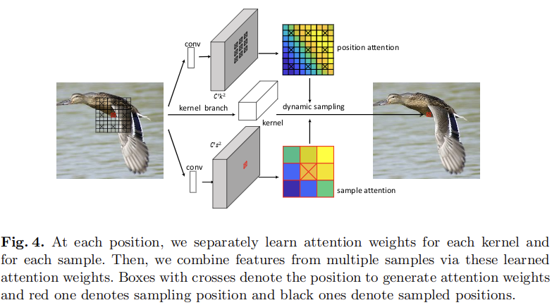
  • In contrast, our attention mechanism aims at combining features from multiple samples via learning weights for each positions’ kernels at each sample.

主要结构

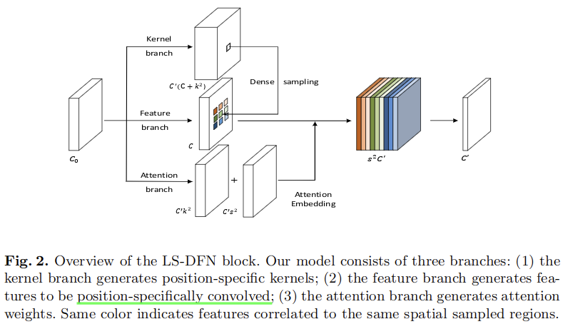
这里展示了网络的核心模块。主要包含是三个分支：kernel branch、feature branch、attention branch。三个分支功能不同，分别用于生成卷积核参数、初步处理了的特征，以及用于加权的注意力权重参数。接下来介绍计算过程。

这里的采样操作要从卷积操作的计算过程说起：

这里表示的是使用第l层的输出作为第l+1层的输入，从而计算对应的输出的过程。从表达式中可以看出来，对于每个输出的(x,y,v)位置而言，都会对应一个输入的kxkxC(k是卷积核大小，C表示输入数据的通道数量)的区域，这个区域中的数据都有自己对应的权重。

• 对于常规的卷积，这里的W是在空间上共享的。也就是随着x,y的变化，这里的W是不变的。
• 对于动态卷积而言，这里的W对于每一个(x,y)位置实际上也是不同的。

要注意，从文章后面来看，这里的x,y表示的并不是对应的k2区域的中心，而应该是这个区域的左上角的元素坐标，通过使用(y+j,x+i)来对整个k2区域进行索引。

Dense Sampling

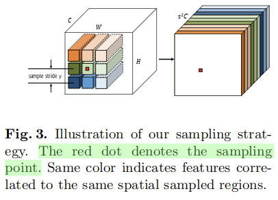
为了获得更大的感受野，和更稳定的梯度，这里使用生成的位置特定的核来卷积处理特征分支生成的特征的对应位置上的特征，还同时采样它们的邻域范围作为额外的特征：

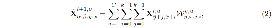
• 这里的W是位置特定的核，是由kernel分支生成的
• 最终的输出每个位置的坐标分别被v、alpha、beta、y、x进行索引，如果设，那么可以得知，该计算输出的X的形状为，将前两维整合，可以得到最终的通道数为
• 。所以可以知道，对于输出的一个位置(x,y)而言，只有一组权重，会用来计算个子区域，各个相邻（上下、左右）子区域中心点的距离为。所以总的采样区域面积是（总体感受野扩大为原来的大约（只是近似）倍）。因此要比原始的位置特定kernel（没有额外的采样区域）处理的样本数据要更多，会得到一个更稳定的梯度
• 当s=1的时候，LS-DFNs就会退化为原始的DFN

这里对于不同区域的采样，感觉可以使用带扩张的 torch.Unfold 实现。

Attention Mechanism

为了在一个位置上融合多个采样区域的结果，一个直接的方法是堆叠个采样特征来形成大小为，另外也可以通过汇集操作（感觉理解上有点像是 torch.Unfold 做的事）。

但是第一种方法，会破坏平移不变性，第二种方法则无法确定哪个采样更重要。为了处理这个问题，这里通过为每个样本的每个位置上的卷积核学习注意力权重，从而使用注意力机制来融合这些特征。由于注意力权重也是位置特定的，所以输出特征的分辨率也就得到了潜在的保留，另外，注意力机制可以从残差学习中获益。

这里在关于(x,y)的计算中，考虑了对应的所有的采样区域，从下标表示可以看出来：

1. i,j迭代的是对应的k2区域内部的，也就是一个卷积核的覆盖范围
2. 这里的注意力权重，实际上针对所有的采样区域都不一样，也就是一次卷积处理，就包含参数个
3. 而卷积核权重参数则是在在所有的采样区域是共享的，都和中心的(x,y)对应的k2区域使用的一致

注意这里的符号表示，使用了波浪线表示注意力加权后的卷积结果。

可以看出来，在上述表示中，需要的注意力权重有个，这对于计算而言比较费时，而且容易导致过拟合（参数过多）。因此这里将其进行分离，不对所有采样区域、所有中心区域使用的权重进行联合的表示，而是拆分成两个部分：

1. 专门学习位置注意力权重
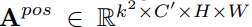
2. 专门学习采样注意力权重

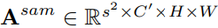
从而参数量变成了。

式子3也变成了：

对于网络实现，这里使用了两个分支来进行两个注意力的预测：

对于采样注意力子分支而言，其包含个输出通道，位置注意力子分支有个输出通道。二者分别用来区分不同位置和不同采样区域之间的相对重要性。进一步的，这里对每个注意力权重手动加1来利用残差学习的优势。

最终通过注意力机制组合不同的采样结果：

也就是对于个区域的结果进行了整合（前一步中已经将注意力权重乘上了）。

Noting that feature maps from previous normal convolutional layers might still be noisy, the position attention weights help to filter such noise when applying largely sampled dynamic filtering to such feature maps. And the sample attention weights indicate how much contribution each neighbor region makes.

Kernel Branch

这里通过使用kernel branch来生成最终使用的卷积核，这是空间相关的。这样的核实现的卷积操作实际上可以看作是一种动态卷积。

对于直接使用性终于传统CNN相同的位置特定核W将会有形状为，由于都是相对较大的值，所以在kernel branch需要的输出通道（）可能变得很大，这会导致极大地计算消耗。最近，几份工作专注于减少核参数，例如MobileNet通过分离卷积核到不同的部分，从而使得CNN更为有效的运行在现代移动设备上。受此启发，这里也进行了类似的操作，以减少参数。

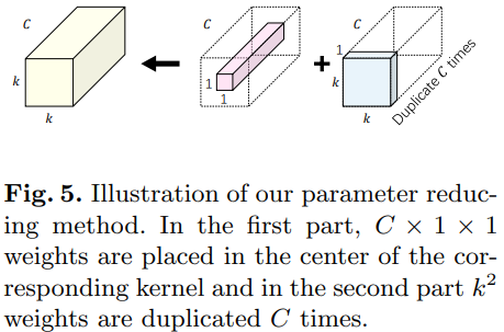
检查层中被激活的输出特征图，通常在通道之间共享相似的几何特征，我们提出了一种新的核结构，将原始核拆分成两个单独的部分以减少参数。正如图5所示：

1. 一方面，对于通道加权，是一个大小的卷积核，在空间上共享，用来模拟通道之间的差异性
2. 另一方面，对于每个位置进行加权，是一个大小的卷积核，在通道上共享，用来模拟通道之间共享的几何特征（shared geometric characteristics）

通过分离卷积核，这里对于每个位置的参数量变成了，而不是原来的。形式上，式子2中的卷积核变成了如下的形式：

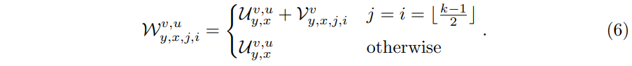
• 对于U的索引有x、y、v、u，而对于V的索引包含x、y、i、j、v
• 对应于式子2中的表示，v表示的是对输出通道的索引，也就是说，输入的每个通道，使用的V都是一致的，而对于每个区域的左上角坐标(x,y)和对应的k2范围内的数据，对应的V的数据是不同的
• 对于U而言，这里针对每个位置(x,y)对应的k2范围，其在输入的空间维度上是共享的，但是通道维度上（由u索引）是不同的
• 由于这里对于i和j的限制，所以V仅是在（也就是对应的中心位置）有效（我怀疑这里是不是写错了，是不是想写在该范围内使用）

式子6中已经基本将权重部分表示清楚了，但是还是需要进一步改进。直接使用6中生成的kernel，这很容易导致在有噪声的真实数据集中导致没法收敛（divergence），原因在于，只有对核分支中的卷积层进行良好的训练，才能使特征分支具有良好的梯度，反之亦然。 因此，很难同时从头开始训练这两个分支。此外，由于卷积核在空间上不共享，所以每个位置处的梯度更有可能是有噪声的，这使得核分支甚至更难训练，进一步阻碍了特征分支的训练过程。

这里通过使用残差学习来解决这个问题，学习恒等卷积核的残差。

这里通过对于卷积的中心位置添加一个1/C，来实现恒等映射。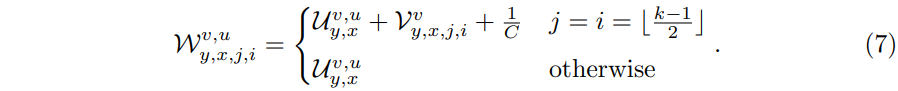

这里在对于输入通道通过索引u进行累加的时候，由于1/C的存在，实际上会出现一个相同权重相加的项，变相实现了恒等映射。但是这个和原始的ResNet的恒等映射略有不同，后者对于原始数据进行了完整的保留，包括数据和数据之间的顺序关系，而这里的设置只是在对输入进行加权求和的时候，使用的相同的权重，相当于计算了均值：

最初，由于核分支的输出接近于零，LS-DFN从特征分支获得近似平均的特征。它保证梯度对于反向传播到特征分支足够可靠。这反过来有利于核分支的训练过程。

实验细节

Object Detection

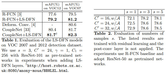
• When applying our LS-DFN, we insert it into object detection networks such as R-FCN and CoupleNet. In particular, it is inserted right between the feature extractor and the detection head, producing C‘ dynamic features. It is noting that these dynamic features just serve as complementary features, which are concatenated with original features before fed into detection head.
• For R-FCN, we adopt ResNet as feature extractor and 7x7 bin R-FCN [7] with OHEM [32] as detection head. During training process, following [4], we resize images to have a shorter side of 600 pixels and adopt SGD optimizer.
• Following [17], we use pre-trained and fixed RPN proposals. Concretely, the RPN network is trained separately as in the first stage of the procedure in [22].
• We train 110k iterations on single GPU with learning rate 10−3 in the first 80k and 10−4 in the next 30k.
• As shown in Table 1, LS-DFN improves R-FCN baseline model’s mAP over 1.5% with only C’ = 24 dynamic features. This implies that the position-specific dynamic features are good supplement to the original feature space.
• And even though CoupleNets [33] have already explicitly considered global information with large receptive fields, experimental results demonstrate that adding our LS-DFN block is still beneficial.

关于运行时分析：Since the computation at each position and sampled regions can be done in a parallel fashion, the running time for the LS-DFN models could have potential of only slightly slower than two normal convolutional layers with kernel size s2.

Semantic Segmentation

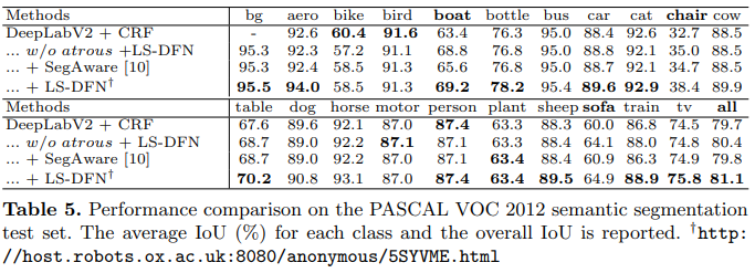
• We adopt the DeepLabV2 with CRF as the baseline model.
• The added LSDFN layer receives input features from res5b layer in ResNet-101 and its output features are concatenated to the res5c layer.
• For hyperparameters, we adopt C‘ = 24, s = 5, γ = 3, k = 3 and a 1×1 256-channel post-conv layer with shared weights at all three input scales.
• Following SegAware [10], we initialize the network with ImageNet model, then train on COCO trainval sets, and finetune on the augmented PASCAL images.

Optical Flow Estimation

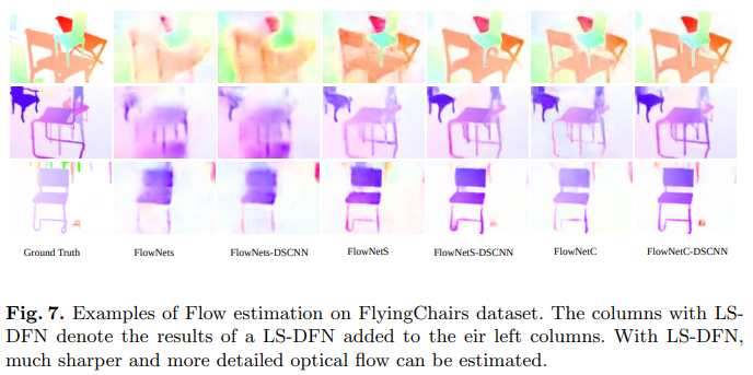
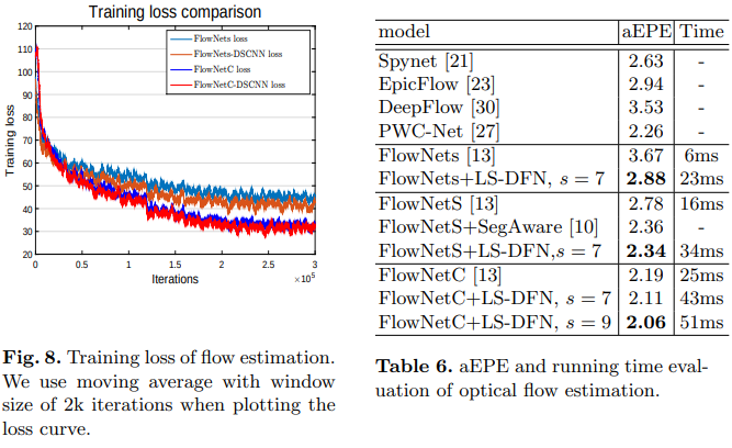
• We perform experiments on optical flow estimation using the FlyingChairs dataset [6]. This dataset is a synthetic one with optical flow ground truth and widely used in deep learning methods to learn the motion information. It consists of 22872 image pairs and corresponding flow fields.
• In experiments we use FlowNets(S) and FlowNetC [13] as our baseline models, though other complicated models are also applicable.
• All of the baseline models are fully-convolutional networks which firstly downsample input image pairs to learn semantic features then upsample the features to estimate optical flow.
• In experiments, our LS-DFN model is inserted in a relative shallower layer to produce sharper optical flow images. Specifically, we adopt the third conv layer, where image pairs are merged into a single branch volume in FlowNetC model. We also use skip-connection to connect the LS-DFN outputs to the corresponding upsampling layer.
• In order to capture large displacement, we apply more samples in our LS-DFN layer. Concretely, we use 7 × 7 or 9 × 9 samples with a sample stride of 2 in our experiments. We follow similar training process in [7] for fair comparison（We use 300k iterations with double batchsize）.
• As shown in Fig. 7, our LS-DFN models are able to output sharper and more accurate optical flow. We argue this is due to the large receptive fields and dynamic position-specific kernels. Since each position estimates optical flow with its own kernels, our LS-DFN can better identify the contours of the moving objects.

相关链接

• 论文：https://arxiv.org/pdf/1803.07624.pdf