arxiv2019年8月9日21:48:09 目前还是放在arxiv上的,具体链接在最后一节中。
这篇文章主要内容:
- 提出一种轮廓损失,利用目标轮廓来引导模型获得更具区分能力的特征,保留目标边界,同时也能在一定程度上增强局部的显著性预测。
- 提出了一种层次全局显著性模块,来促使模块逐阶段获取全局内容,捕获全局显著性。
网络结构
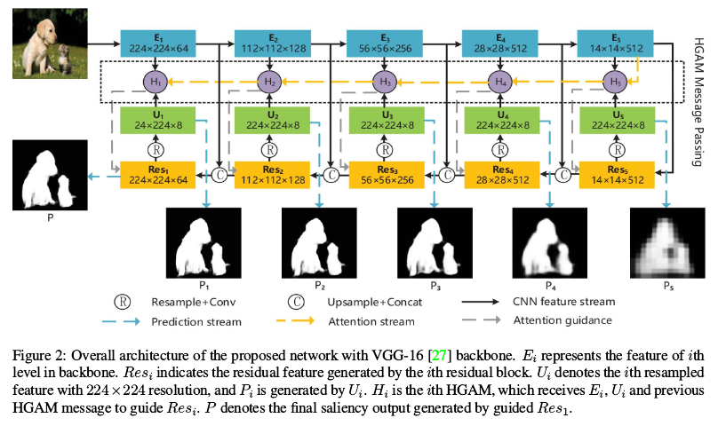
- 是一个FPN-like的结构
- Ei表示第i个编码器模块的输出特征,所有的这些特征集合表示为FE
- 每个编码器都使用了一个残差结构来集成多尺度特征,解码器将Ei转化为Resi,所有这些特征集合表示为FR
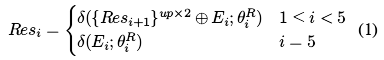
- 这里的
 表示的是对应关系,而非相减的操作
 - 这里的
 表示卷积层,
 表示卷积层参数
  表示concat,
 表示上采样两倍
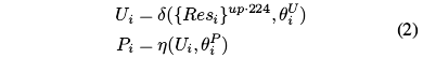
- 为了实现深监督,这里对于每个Resi,直接上采样到224x224,获得Ui,再通过使用sigmoid激活的卷积层来获得显著性预测Pi
- 训练时使用五个层级的损失,但是对于**各级使用了不同的权重**
Contour Loss
由于对于显著性目标检测(这里与“分割”无异)的每个样本的密集预测来说,实际上在边界附近的像素可以看作是一些难样本,参考Focal Loss的设计,在交叉熵上使用空间加权,来对显著性目标边界的像素的结果设置更高的权重。空间权重可以表示为下式对应的集合。
 表示膨胀炒作,
 表示腐蚀操作,都是用的5x5的核S实施的
- K是一个超参数,这里论文设定为5
- Gauss是为了赋予接近边界但是并没有位于边界上的像素一些关注,这里对于Gauss的范围设置为5x5
- 这里的
 表示像素224x224这样的整个图上的像素,是否是远离边界,是的话就是1,反之为0
 - Compared with some boundary operators, such as Laplace operator, the above approach can generate thicker object contours for considerable error rates.
- 整体损失函数设置如下:
- 这里论文里的描述应该有误,M是权重,Y是真值,Y*是预测
- 实际中,对于式子(3)中的loss,对应的就是(5)中对应层级的LC
Hierarchical Global Attention Module
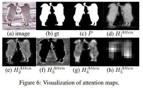
认为现有的显著性检测方法大多是基于softmax函数的:which enormously emphasizes several important pixels and endows the others with a very small value. Therefore these attention modules cannot attend to global contexts in high-resolution, which easily lead to overfitting in training.
因此,这里使用了一个新的基于全局对比度的方法来利用全局上下文信息。这里使用了特征图的均值来作为一个标准:Since a region is conspicuous infeature maps, each pixel in the region is also significant with a relatively large value, for example, over the mean. In other words, the inconsequential features often have a relatively small value in feature maps, which are often smaller than the mean. 于是使用特征图减去均值,正值表示显著性区域,负值表示非显著性区域。于是可以得到如下的分层全局注意力:
- 这里的FIn表示输入的特征,Aver和Var表示对应于FIn的均值和方差值
 表示一个正则项,这里设定为0.1
 是一个小数,防止除零
- Compared with softmax results, the pixel-wise disparity of our attention maps is more reasonable, in other words, our attention method can retain conspicuous regions from feature maps in high-resolution
这里通过提出一个hierarchical global attention module (HGAM) 来捕获multi-scale global context。
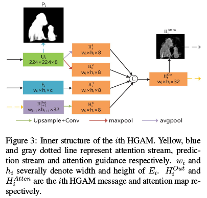
- 这里作为输入的有三部分:来自本级的上采样特征Ui;来自本级的编码器特征Ei,以及来自上一级的HGAM信息Houti+1
- 为了提取全局上下文新西,这里对于Ui使用了最大池化和平均池化处理,获得H1和H2,这里来自于[Cbam: Con-volutional block attention module]
- 对于Ei和Houti+1调整通道和分辨率分别获得H3和H4
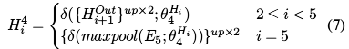
- HAtten可以通过(6)获得
- Houti用于生成下一个Houti+1,而HAtten用来引导残差结构:

- 这里的
 表示像素级乘法
 - 所以最终的预测输出实际上是ResG1生成的P
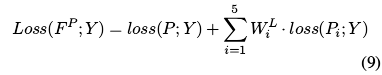
- 总体的训练损失改进为:
实验细节
- Our experiments are based on the Pytorch framework and run on a PC machine with a single NVIDIA TITAN X GPU (with 12G memory).
- For training, we adopt DUTS-TR as training set and utilize data augmentation, which resamples each image to 256×256 before random flipping, and randomly crops the 224×224 region.
- We employ stochastic gradient descent (SGD) as the optimizer with a momentum (0.9) and a weight decay (1e-4).
- We also set basic learning rate to 1e-3 and finetune the VGG-16 backbone with a 0.05 times smaller learning rate.
- Since the saliency maps of hierarchical predictions are coarse to fine from P5 to P1, we set the incremental weights with these predictions. Therefore WL5, …, WL1 are set to 0.3, 0.4, 0.6, 0.8, 1 respectively in both Eq 3 and 9.
- The minibatch size of our network is set to 10. The maximum iteration is set to 150 epochs with the learning rate decay by a factor of 0.05 for each 10 epochs.
- As it costs less than 500s for one epoch including training and evaluation, the total training time is below 21 hours.
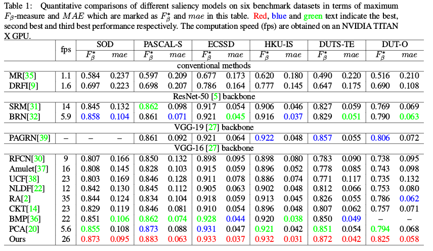
- For testing, follow the training settings, we also resize the feeding images to 224×224, and only utilize the final output P. Since the testing time for each image is 0.038s, our model achieves 26 fps speed with 224×224 resolution.
参考链接

若有收获,就点个赞吧
0 人点赞
