cvpr2017的论文。提出一种弱监督的显著性检测方法。
主要工作
在图像分类任务的基础上构建了显著性检测的结构。文章仅仅使用了ImageNet Det的数据来作为数据集,仅有多类别标记,并没有使用其他的真值。所以难点在于如何通过这些Image-level的监督实现更好的密集预测——显著性检测。
文章的主要贡献包含以下几个方面:
- 较早开始以弱监督的角度研究显著性检测任务的工作
- 提出了一种新的全局池化方法——全局平滑池化
- 使用生成的显著性图预测作为训练显著性部分的真值,实现了一种“自训练”
- 对于显著性真值进行细化,对于条件随机场的计算进行了调整,使其可以增强空间标记的一致性
- 提出了一个新的数据集——DUTS
主要结构
结构流程
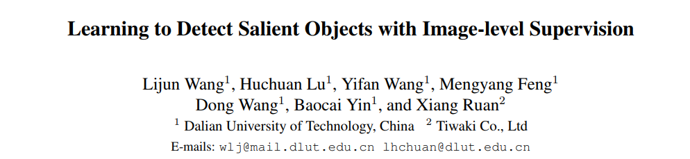
- 输入图像,也就是图4中的a
- 通过共享的VGG16的卷积层(也就是图4中的b)得到最深处的特征和几处侧输出(这里的VGG-16的卷积层仅保留了四个池化层)
- 关于使用的FCN和FIN这里没有画出来
- FCN包含一个Conv-BN-ReLU结构,FCN没有直接预测目标得分图,而是生成了中间得分图(intermediate score map,也就是图4中的c),其包含512个通道,这对应着一些类别无关的中级模式
- FIN包含一个Conv-BN-Sigmoid结构,用来产生显著性图F,也就是图4中的d,这被用来作为得分图的掩膜,以获取masked score map,也就是图4中的e
- 对于得到的masked score map通过重新构造的GSP(global smooth pooling)层整合空间响应到512维的图像级得分,这将被后续的全连接层用来生成200维的针对目标类别的得分矢量,最后通过sigmoid层得到各个类别的概率
这里可以认为是一个多标签分类问题: 多标签问题与二分类问题关系在上文已经讨论过了,方法是计算一个样本各个标签的损失(输出层采用sigmoid函数),然后取平均值。把一个多标签问题,转化为了在每个标签上的二分类问题。
- https://juejin.im/post/5b38971be51d4558b10aad26
- https://yuanxiaosc.github.io/2018/07/01/%E4%BA%8C%E5%88%86%E7%B1%BB%E3%80%81%E5%A4%9A%E5%88%86%E7%B1%BB%E4%B8%8E%E5%A4%9A%E6%A0%87%E7%AD%BE%E9%97%AE%E9%A2%98%E7%9A%84%E5%8C%BA%E5%88%AB%E2%80%94%E2%80%94%E5%AF%B9%E5%BA%94%E6%8D%9F%E5%A4%B1%E5%87%BD%E6%95%B0%E7%9A%84%E9%80%89%E6%8B%A9/
GSP
使用Image-level标注的训练集 。网络分类的分支使用的输出表示为
 ,最终与l进行交叉熵的计算。Although the CNN is trained on image-level labels, it has been shown that higher convolutional layers are able to capture discriminative object parts and serve as object detectors. However, the location information encoded in convolutional layers fails to be transferred to fully connected layers. 这里共享的CNN的部分的基础上添加了一层卷积层,为了使用image-level标注的真值,这里需要一些集成的手段,来将FCN(也就是附加的一层卷积层)的密集预测输出进行整合,也就是将像素级得分图S转化为image-level的得分矢量s,这是通道独立的。
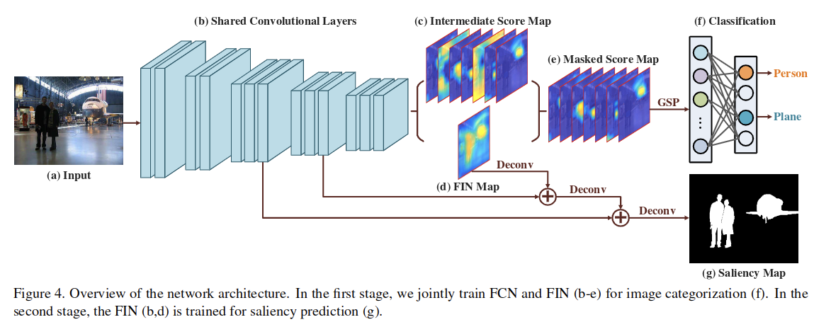
常用的方法有全局最大池化GMP和全局平均池化GAP。这里主要分析了二者各自的问题:
- 对于GMP,对于每个通道而言,只有最大响应的位置的值被考虑到。考虑到更高层的卷积层表现更像是目标检测器,可以将得分图作为一个对这些检测器的集成的一个空间响应,这就可以说,GMP只会关注单个的响应,检测器仅使用最具有判别性的目标部分进行训练。结果,大多无法发现对象的完整扩展。
- 对于GAP,所有的位置的响应都被赋予相同的权重值,鼓励检测器对于所有的空间位置有着相同的响应,这是不合理的,并导致对物体区域的高估(overestimated)。
GMP的缺点主要是因为对于最高响应的选择的“硬”选择造成的,这也就涉及到了非平滑的最大值问题,可以通过平滑这个选择操作在很大程度上解决这个缺点。最终使用Smooth minimization of non-smooth functions中的方法,来平滑最大值操作,也就是通过对特征取最大的操作减去一个关于取最大操作的权重矢量的强凸函数来平滑。这里使用L2范数: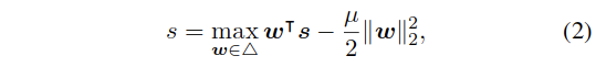
当没有后面的强凸函数进行约束时,which can be simply solved by setting the weight of the highest response to 1, while others to 0. 有了这个约束,可以对于原来的1/0这样的结果并不能取得最大值,因为这时的约束项也是最大的(要注意这类的约束项),要注意w之和为1:
,
,是一个概率单纯形。
这里的 表示权衡的参数。可以看到:
- As μ approximates 0, (2) is reduced to GMP.
- When μ is sufficiently large, the maximization of (2) amounts to the minimization of ||w||22 , and requires each element of w equals to 1/d, which has the same effect of GAP.
Since the L2 norm of the weight w does not explicitly contain information of feature responses, we omit this term in the aggregated response s and only use (2) to determine the weight. It turns out that the optimal weight  can be computed by a projection of feature s onto the simplex (3).
概率单纯形:对于一个n-1-单纯形,其内部包含n维矢量的所有元素值均为非负数,且各元素之和为1。 0-单纯形为点;1-单纯形为线段;2-单纯形为三角形;3-单纯形为四面体……
提出的GSP可以表示为如下两步: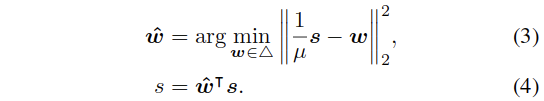
具体转化过程见论文,这部分确实不是太懂。
The proposed GSP is motivated by two insights.
- Firstly, by smoothing GMP, GSP jointly considers multiple high responses instead of a single one at each time, which is more robust to noisy high responses than GMP and enables the trained deep model to better capture the full extend of the objects rather than only discriminative parts.
- Secondly, as opposed to GAP, GSP selectively encourages the deep model to fire on potential object regions instead of blindly enforcing high response at every location. As a result, GSP can effectively suppress background responses that tend to be highlighted by GAP.
FIN
When jointly trained with GSP layer on the image-level tags, the score map S generated by FCN can capture object regions in the input image, with each channel corresponding to an object category. For saliency detection, we do not pay special attentions to the object category, and only aim to discover salient object regions of all categories.
To obtain such a category-agnostic saliency map, one can simply average the category score map across all the channels. However, there are two potential issues.
- Firstly, response values in different channels of the score map often subject to distributions of different scales. By simply averaging all the channels, responses in some objects (parts) will be sup-pressed by regions with higher responses in other channels.
- In consequence, the generated saliency maps either suffer from background noises or fail to uniformly highlight object regions.
- 更重要的是,由于得分图的每个通道都经过训练以捕捉训练集的特定类别,因此很难泛化到看不见的类别。
Foreground Inference Net (FIN)设计来处理上述问题,集成得分图S的类别特定的响应。其将图像X作为输入,预测一个下采样16倍的显著性图。通过最终的sigmoid,每个元素值被缩放到0~1之间。
由于本文是半监督方法,所以没真值来训练FIN,这里和另外的用于生成中间得分图的FCN结构一起联合训练。
对于输入的X,FIN得到F,是一个单通道的nxn的二维张量,FCN得到一个C通道的nxn的三维张量。使用F作为S的掩膜进行处理:
这里表示了S的第k个通道的计算,实际上各个通道都要进行计算。这里的处理后的得分图hatS之后使用GSP处理后得到了image-level的得分矢量hats。
对于FIN和FCN的联合训练,是通过最小化损失函数下式进行的: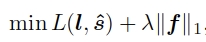
这里的L表示交叉熵。
The key motivation is as follows. Each channel of the score map S highlights the region of one object category by spatial high responses. To preserve these high responses in the masked score map hatS, the saliency map F is required to be activated at object regions of all categories…we aim at learning FIN to automatically infer saliency maps of all categories using weak supervision
这里对损失添加了一个正则项,但是这里使用的是输出的得分图F的矢量结果的L1范数。这主要是担心FIN会学习在所有位置都有高响应的微不足道的解决方案。
- The first term encourages F to have high responses at foreground, while the second term penalizes high responses of F at background; λ is a pre-defined trade-off parameter.
- Note that the regularization term in (6) is imposed on the feature representations rather than the weight parameters, which is reminiscent of a recent work [12], where L1 regularization on feature is used to enforce better generalization from low-shot learning. In contrast, we aim to produce ac-curate saliency maps with less background noise.
另一个挥之不去的担忧是,在一组固定的类别上训练的FIN可能难以泛化到为看不见的类型。
To address this issue, we apply the masking operation (5) to the intermediate score map rather than the final one. The intermediate score map does not directly correspond to object categories, As con-firmed by [11], it mainly encodes mid-level patterns, e.g., red blobs, triangular structures, specific textures,etc., which are generic in characterizing all categories.
Consequently, FIN can capture conspicuous regions of category-agnostic objects/parts and can better generalize to unseen categories
训练过程
使用Image-level的tags进行预训练
**
- 获得Image-level标注的训练集,这里包含着N个样本,以及对应的类别标注矢量l
- 权重使用预训练的VGG模型,其它层使用随机初始化(使用Delving deep into rectifiers: Surpassing human-level performance on imagenet classification的方法)
- 所有的输入图像都被放缩到固定的256x256大小
- 对于FIN而言,其总体的步长是16像素(因为前面有4个最大池化),这会使得输出的显著性图只有16x16大小
- 使用SGD,batchsize为64,momentum为0.9,学习率初始化为0.01,并且每隔20个epoch衰减0.1倍
- 通过最小化以下目标函数来训练网络:
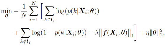
这里的 表示网络参数,其中第一项和第二项是交叉熵损失,来衡量预测的准确率,第三项表示针对预测的显著性图f的L1正则项,而最后一项表示权重衰减的约束。其中的超参数
 、
、 、设置为5e-4和1e-4,以及10。
使用估计的像素级标记进行self-training
**
在预训练之后,FIN会生成粗略的显著性图,这已经捕获了前景区域。开始进行第二步训练,通过迭代两步来优化预测:
- 使用训练好的FIN来估测真值显著性图作为真值
- 使用获得的估测的显著性图真值来微调FIN
为了提升输出的分辨率,这里扩展了FIN的结构:
- 在第14层卷积层的顶部,构建了三个额外的转置卷积层,使用上采样x2、x2、x4按照图4所示结构,恢复了原始分辨率,同时也组合了low-level以及high-level的特征
- 使用了两个额外的技术保证了估计的真值的质量:
- 使用提出的CRF结构进行细化
- 使用对于标签噪声比较稳健的bootstrapping loss训练
使用提出的CRF结构进行细化
输入图像先通过Structured forests for fast edge detection超像素算法进行分割,划分为超像素集合 ,每个超像素的特征表示为自身的平均的RGB和LAB特征。根据FIN估计的显著性图F,如果超像素内部的平均显著性值大于0.5,则对应的超像素标记为前景(
 )。
)。
Two Gaussian Mixture Models (GMMs) are learned to model the foreground and background appearance, respectively, with each GMM containing K=5 components. To refine the saliency labels  , a binary fully connected CRF is defined over these labels with the following energy function E. 其中
 中的w表示GMM的参数。
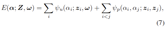
基于超像素的一元项定义如下,这里的p(zi|wai)表示超像素zi属于前景或者背景的概率:
而二元项可以表示为: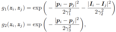

- 这里的
 表示指示函数
 - g1和g2是测量相似性的高斯核,权重为两个

 和
和 表示的是超像素z对应的颜色特征和位置
- 所有的超参数都按照Efficient inference in fully connected crfs with gaussian edge potentials进行设置
Conventional CRFs find the optimal label set α* to solve the energy function. In comparison, we propose an EM-like procedure by iteratively updating the GMM parameter ω and the optimal label set α.
- Given the current optimal α*, we minimize (7) by learning parameter ω of foreground and background GMMs;
- when ω is fixed, we optimize (7) via mean field based message passing to obtain α*.
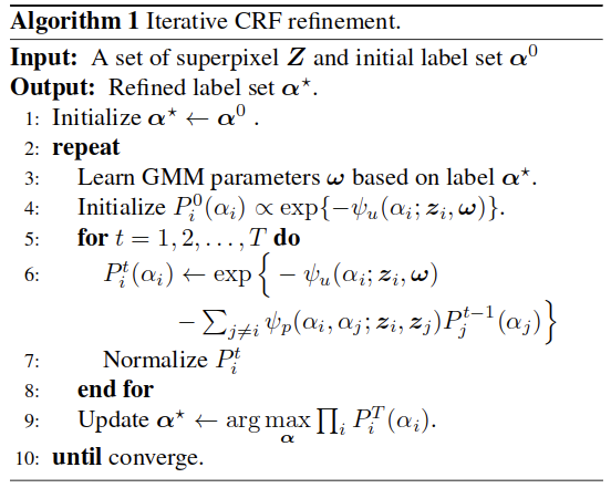
The number of iteration is set to 5 in all experiments. In each iteration, message passing is conducted for T = 5 times. By jointly updating GMMs and labels, our algorithm is more robust to initial label noise, yielding more accurate refinement. After refinement, we assign the label of each superpixel to all its pixels to obtain a refined saliency map R.
**
使用bootstrapping loss对FIN进行微调
使用细化后的显著性图R作为估计的真值来微调扩展后的FIN。这里为了降低噪声的影响,使用了bootstrapping loss[TRAINING DEEP NEURAL NETWORKS ON NOISY LABELS WITH BOOTSTRAPPING]来进行训练: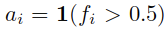
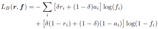
这里的r是向量化的真值R,f是扩展后的FIN的向量化的输出显著性图F。这里的i是像素级索引。这里的权重参数 根据原论文设定,被固定位0.95。The bootstrapping loss is derived from the cross-entropy loss, and enforces label consistency by treating a convex combination of i) the noisy label ri, and ii) the current prediction ai of the FIN, as the target.
We solve the loss function using mini-batch SGD, with a batch size of 64. The learning rates of the pre-trained and newly-added layers of FIN are initialized as 1e-3 and 1e-2, respectively, and decreased by 0.1 for every 10 epochs.
In practice, the self-training starts to converge after two iterations of “ground truth estimation”–”fine-tuning”. **
实验细节
相关链接

若有收获,就点个赞吧
0 人点赞
