图片 - Attentive Feedback Network for Boundary-Aware Salient Object Detection - 《深度学习论文阅读》

网络结构
主要亮点
实验细节
相关链接

网络结构

主要亮点

问题清晰明确，重点解决边界模糊的问题
使用最大池化实现了膨胀腐蚀操作，从而得到边界注意力图
边界增强损失（Boundary Enhanced Loss）
新的全局感知模块，使用分块堆叠后的卷积实现全局视野

明确的目标

文章反复都在提一个问题，那就是现有CNN方法进行显著性检测时的一个通病，那就是边界的模糊问题。虽然也有想CRF这样的技术来进行一定的增强，但是却也在一定程度上增加了计算消耗，需要更多的计算时间。

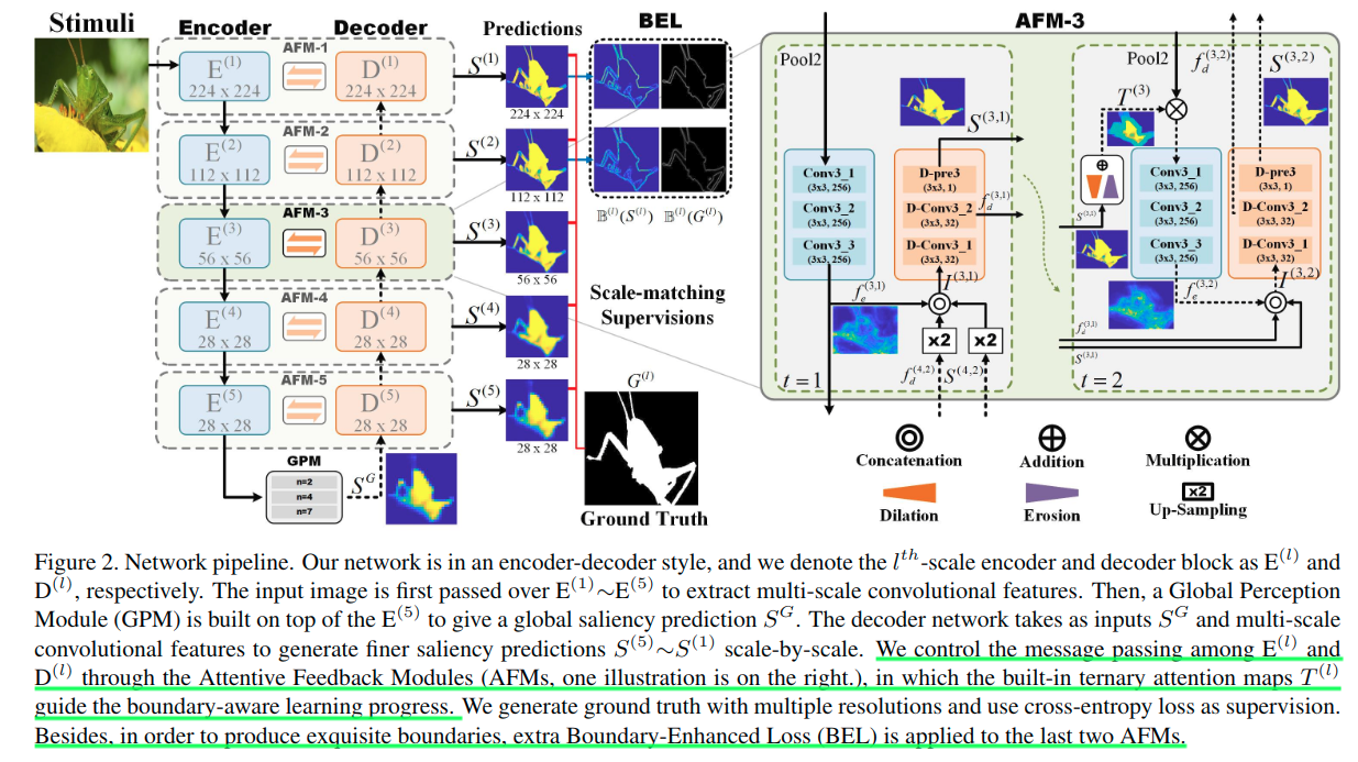
文章引入了通过采用每个编码器块和相应的解码器块来构建的注意反馈模块（AFM），以逐比例地细化粗略预测。注意力反馈模块有助于捕捉目标的整体形状。此外，边界增强损失（BEL）用于产生精美的边界，帮助在目标轮廓上的显着性预测的学习。提出的模型具有学习生成精确和结构完整的显着性目标检测结果的能力，同时，可以在不进行后处理的情况下明确切割目标的轮廓。

注意力反馈模块

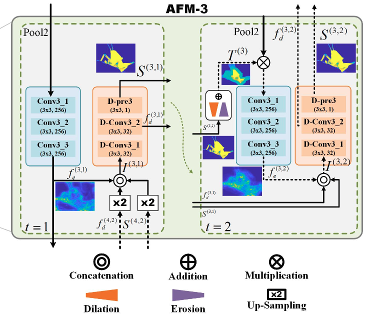
这里以AFM-3为例，这个是位于第三阶段的编码器与解码器之间的一个模块，要注意图中不同位置的编号，右上角括号中的第一个数字表示的是来自第几个阶段的特征。可以看到，本模块（包含编码器与解码器的对应阶段）的计算是要使用来自更高阶段的信息的，以实现信息的恢复。橙色的部分是解码器的操作，而青色的部分是编码器的操作。

这里涉及到了一个迭代的过程，分为两个时间步。但是，在第一个时间步骤细化之后，无法保证结果的质量，因为前一个块的引导涉及一个向上扩展操作，它会引入许多不准确的值，特别是在对象边界上。除此之外，假设前一个区块未能分割出整个目标，后续区块将永远不会有机会执行结构上完整的检测。AFM在第二时间步中的反馈流中使用三元注意力图提供了纠错的机会。

第一个时间步按照t=1指示的操作处理
而t=2时刻则是使用了一个自注意力的处理，这里是将t=1预测出来的显著性图S，分别通过下面公式所示的膨胀腐蚀两种操作之后，二者平均之后获得的注意力图。
1. 三元注意力图T计算为D和E的均值。因此缩减后（腐蚀）的显着区域的像素值接近1，而边界附近得分接近0.5。剩下的区域（背景）几乎为0。
2. 因此，当t = 2时，通过在S上操作膨胀腐蚀来产生三元注意力图T——指示相同的背景，自信的前景和不确定的（边界）区域。

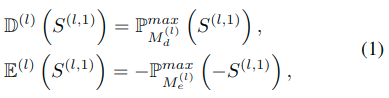
这里的膨胀腐蚀使用的是最大池化操作，具体参数（池化核）见后表。

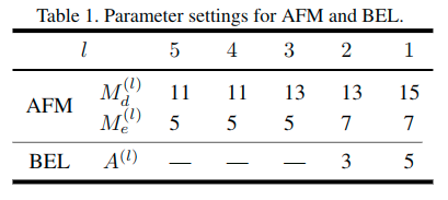
AFM的设置和对应与边界增强损失的设置。

These parameters are adjusted following the observations:

for predictions with low-resolution, the ternary attention map should involvein enough regions in case of excluding the target object. Thus the kernel size should be relatively large to the spatialsize. With the increasing of spatial resolution, we could decrease the kernel size cause the overall shape of targets could be recognized already
the kernel size of the Erosion M should be smaller than the kernel sizeof the Dilation M because that we need to perceive as much as possible details around the boundary regions.

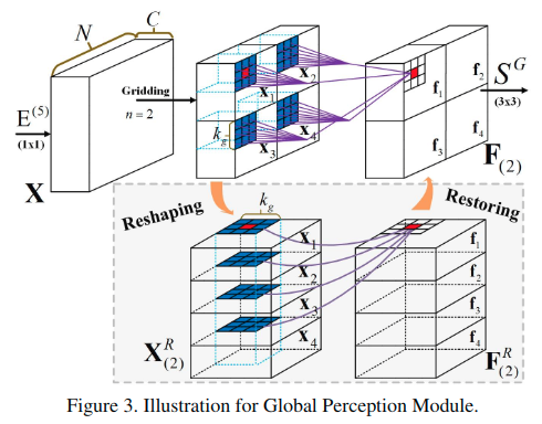
全局感知模块

至于全局显着性预测，[Dhsnet: Deep hierarchical saliency network for salient object detection]在其全局视图CNN中直接使用全连接层。问题是：

最深层中的相邻元素具有大的重叠感受域，意味着输入图像上的相同像素贡献了大量冗余次数来计算单个显着性值
使用所有像素，对于确定一般位置很有用，但局部模式会丢失

这些事实激励了全局感知模块的提出，以充分利用局部和全局信息。从图中可以看出来，这里考虑了局部的邻居。通过这种方式，可以同时保证局部模式和全局信息。最终整个模块使用了多个尺度的划分，包括n=2/4/7，也就是划分成2x2/4x4/7x7三个不同的分支，进行堆叠重组后进行kgxkg的卷积，最终使用一个3x3卷积处理恢复后的特征得到预测的显著性图。

**
全局感知模块在图中绘制的很详细。就是在拆分并堆叠之后的特诊图上进行一般的卷积，进而实现了对于全局信息的利用。关键是这里的实现，不能直接用reshape操作处理，而应该考虑如何进行分割堆叠的处理。pytorch中可以考虑使用chunk和cat的操作。

这里简单写了下这个模块。

2020年12月16日16:16:35补充：这个模块可以借助einops这个库非常简单来实现。

# -*- coding: utf-8 -*-
# @Time    : 2020/12/16
# @Author  : Lart Pang
# @GitHub  : https://github.com/lartpang
import time
import einops.layers.torch as pt_einops
import torch
import torch.nn as nn
class BasicConv2d(nn.Module):
    def __init__(self, in_planes, out_planes, kernel_size, stride=1, padding=0, dilation=1, groups=1, bias=False):
        super(BasicConv2d, self).__init__()
        self.basicconv = nn.Sequential(
            nn.Conv2d(
                in_planes,
                out_planes,
                kernel_size=kernel_size,
                stride=stride,
                padding=padding,
                dilation=dilation,
                groups=groups,
                bias=bias,
            ),
            nn.BatchNorm2d(out_planes),
            nn.ReLU(inplace=True),
        )
    def forward(self, x):
        return self.basicconv(x)
class GPMV1(nn.Module):
    def __init__(self, in_C, out_C, ns=(2, 4, 7)):
        super(GPMV1, self).__init__()
        self.ns = ns
        self.ms = nn.ModuleList(
            [
                nn.Sequential(
                    pt_einops.Rearrange("bs c (g_h h) (g_w w) -> bs (g_h g_w c) h w", g_h=n, g_w=n),
                    BasicConv2d(in_C * n * n, in_C * n * n, 3, 1, 1),
                    pt_einops.Rearrange("bs (g_h g_w c) h w -> bs c (g_h h) (g_w w)", g_h=n, g_w=n),
                )
                for n in ns
            ]
        )
        self.fuse = BasicConv2d(len(ns) * in_C, out_C, 1)
    def forward(self, x):
        assert all([x.size(2) % n == 0 for n in self.ns])
        return self.fuse(torch.cat([m(x) for m in self.ms], dim=1))
class GPM(nn.Module):
    def __init__(self, in_C, out_C, ns=(2, 4, 7)):
        super(GPM, self).__init__()
        self.ns = ns
        self.ms = nn.ModuleList([BasicConv2d(in_C * n * n, in_C * n * n, 3, 1, 1) for n in ns])
        self.fuse = BasicConv2d(len(ns) * in_C, out_C, 1)
    def forward(self, in_feat):
        assert all([in_feat.size(2) % n == 0 for n in self.ns])
        feats = []
        for idx, n in enumerate(self.ns):
            chunk_feats = torch.cat(
                [y for x in in_feat.chunk(chunks=n, dim=2)
                 for y in x.chunk(chunks=n, dim=3)], dim=1
            )
            # chunk_feats_v1 = einops.rearrange(in_feat,
            #                                   "bs c (g_h h) (g_w w) -> bs (g_h g_w c) h w",
            #                                   g_h=n, g_w=n)
            # print(torch.all(chunk_feats == chunk_feats_v1))  # => True
            chunk_feats = self.ms[idx](chunk_feats)
            total_feat = torch.cat(
                [torch.cat(x.chunk(chunks=n, dim=1), dim=3)
                 for x in chunk_feats.chunk(chunks=n, dim=1)], dim=2
            )
            # total_feat_v1 = einops.rearrange(chunk_feats,
            #                                  "bs (g_h g_w c) h w -> bs c (g_h h) (g_w w)",
            #                                  g_h=n, g_w=n)
            # print(torch.all(total_feat == total_feat_v1))  # => True
            feats.append(total_feat)
        return self.fuse(torch.cat(feats, dim=1))
if __name__ == "__main__":
    a = torch.rand((4, 32, 28, 28))
    # print(a.mean((0, 1, 2)))
    start = time.time()
    gpm = GPM(32, 32, ns=(2,))
    print(gpm(a).mean((2, 3)), time.time() - start)
    start = time.time()
    gpmv1 = GPMV1(32, 32, ns=(2,))
    print(gpmv1(a).mean((2, 3)), time.time() - start)

损失函数

从结构图中可以看出来。在最后的两个解码器阶段使用了额外的边界监督，使用了一个边界增强损失，这里使用了均值滤波操作，也就是平均池化操作。其核大小设定可见“注意力反馈模块”小节中的表格。

这里使用了平均池化来实现边界轮廓的提取。作差后通过绝对值操作进而提取了边界。

总的损失函数可以表示为：

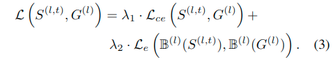
对于各个阶段的显著性图与真值之间使用交叉熵，而边界使用的L2损失（欧式损失），第3/4/5阶段只包含第一项。这是因为这些层不能保持恢复精美轮廓所需的细节。通过从显着性预测本身中提取边界，边界增强损失增强了模型以在边界上进行更多努力。

这一点在CPD论文中也提到了，前三层起码还保留着一些边缘信息，再高层的就更加抽象模糊了。

对于混合项的系数，lambda1:lambda2=1:10。

实验细节

We train our model on the training set from DUTS and test on its test set along with other four datasets.
- ECSSD, PASCAL-S, DUT-OMRON, HKU-IS and DUTS.
文章评估的时候，使用了四个显著性检测指标：PR曲线、F-measure、MAE、S-measure
- S-measure[Structure-measure: ANew Way to Evaluate Fore-ground Maps]，它可以用来评估非二值前景图。同时评估显着性图和真实标注之间的region-aware and object-aware structural similarity。
We do data augmentation by horizontal- and vertical-flipping and image cropping to relieve over-fitting inspired by Liu et al. [21].
When fed into the AFNet, each image is warped to size 224x224 and subtracted using a mean pixel provided by VGG net at each position.
Our system is built on the public platform Caffe and the hyper-parameters are set as follows:
- We train our network on two GTX 1080 Ti GPUs for 40K iterations, with a base learning rate (0.01), momentum parameter (0.9) and weight decay (0.0005).
- The mini-batch is set to 8 on each GPU.
- The ‘step’ policy with gamma = 0.5 and stepsize = 10K is used.
- The parameters of the first 13 convolutional layers in encoder network are initialized by the VGG-16 model and their learning rates are multi-plied by 0.1.
- For other convolutional layers, we initialize the weights using “gaussian” method with std = 0.01.
- The SGD method is selected to train our neural networks.

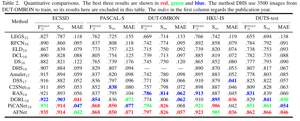
对比其他方法

全局感知模块的配置比较

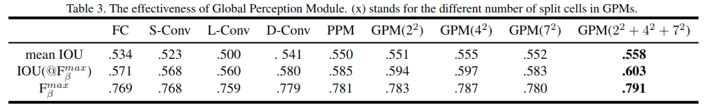
FC: fully-connected layer; S-Conv: convolutional layer with small kernels (3x3); L-Conv: convolutional layer with large kernels (7x7); D-Conv: dilated convolutional layer with small kernels (3x3) and large rates (rate=7); PPM: pyramid pooling module in PSPNet

这里的第二个指标指的是针对于求解maxF时使用的阈值下的二值图得到的IOU，而meanIOU则是平均（应该是所有阈值下结果的平均）的IOU结果。

模块消融

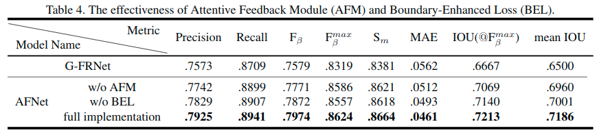
模块效果比较，并且与一个之前的方法[Gated feedback refinement network for dense image labeling]的模型G-FRNet进行了比较。

Attentive Feedback Network for Boundary-Aware Salient Object Detection