主要结构
In this paper, we propose a novel saliency detection method, which contains:
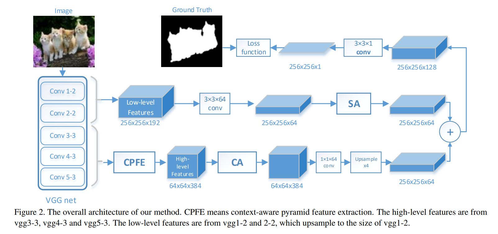
- a context-aware pyramid feature extraction module and a channel-wise attention module to capture context-aware multi-scale multi-receptive-field high-level features
- a spatial attention module for low-level feature maps to refine salient object details and an effective edge preservation loss to guide network to learn more detailed information in boundary localization.
有意思的地方:
- 低级特征上使用了空间注意力模块。
- 高级特征上使用了通道注意力模块和类ASPP结构CPFE。
两种注意力没必要一定要放在一起,反而这里在保留了更多的结构信息的较低层的特征上使用了空间注意力,而在较高层的富含语义信息的特征上使用了CPFE和通道注意力,使用多尺度的感受野和通道加权,更好的使用特征,区分前景背景信息。
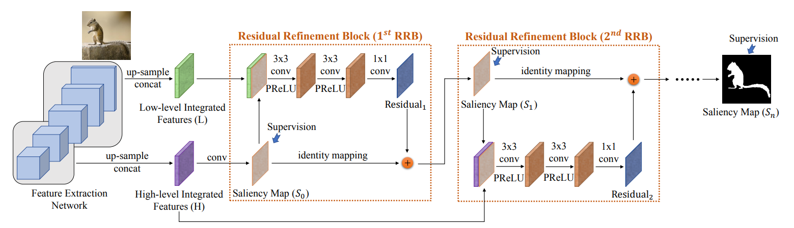
下面是R3Net的结构图,关于这里的拼接组合有些类似。
整体模型的代码:
def VGG16(img_input, dropout=False, with_CPFE=False, with_CA=False, with_SA=False, droup_rate=0.3):# Block 1x = Conv2D(64, (3, 3), activation='relu', padding='same', name='block1_conv1')(img_input)x = Conv2D(64, (3, 3), activation='relu', padding='same', name='block1_conv2')(x)C1 = xx = MaxPooling2D((2, 2), strides=(2, 2), name='block1_pool')(x)if dropout:x = Dropout(droup_rate)(x)# Block 2x = Conv2D(128, (3, 3), activation='relu', padding='same', name='block2_conv1')(x)x = Conv2D(128, (3, 3), activation='relu', padding='same', name='block2_conv2')(x)C2 = xx = MaxPooling2D((2, 2), strides=(2, 2), name='block2_pool')(x)if dropout:x = Dropout(droup_rate)(x)# Block 3x = Conv2D(256, (3, 3), activation='relu', padding='same', name='block3_conv1')(x)x = Conv2D(256, (3, 3), activation='relu', padding='same', name='block3_conv2')(x)x = Conv2D(256, (3, 3), activation='relu', padding='same', name='block3_conv3')(x)C3 = xx = MaxPooling2D((2, 2), strides=(2, 2), name='block3_pool')(x)if dropout:x = Dropout(droup_rate)(x)# Block 4x = Conv2D(512, (3, 3), activation='relu', padding='same', name='block4_conv1')(x)x = Conv2D(512, (3, 3), activation='relu', padding='same', name='block4_conv2')(x)x = Conv2D(512, (3, 3), activation='relu', padding='same', name='block4_conv3')(x)C4 = xx = MaxPooling2D((2, 2), strides=(2, 2), name='block4_pool')(x)if dropout:x = Dropout(droup_rate)(x)# Block 5x = Conv2D(512, (3, 3), activation='relu', padding='same', name='block5_conv1')(x)x = Conv2D(512, (3, 3), activation='relu', padding='same', name='block5_conv2')(x)x = Conv2D(512, (3, 3), activation='relu', padding='same', name='block5_conv3')(x)if dropout:x = Dropout(droup_rate)(x)C5 = xC1 = Conv2D(64, (3, 3), padding='same', name='C1_conv')(C1)C1 = BN(C1, 'C1_BN')C2 = Conv2D(64, (3, 3), padding='same', name='C2_conv')(C2)C2 = BN(C2, 'C2_BN')if with_CPFE:C3_cfe = CFE(C3, 32, 'C3_cfe')C4_cfe = CFE(C4, 32, 'C4_cfe')C5_cfe = CFE(C5, 32, 'C5_cfe')C5_cfe = BilinearUpsampling(upsampling=(4, 4), name='C5_cfe_up4')(C5_cfe)C4_cfe = BilinearUpsampling(upsampling=(2, 2), name='C4_cfe_up2')(C4_cfe)C345 = Concatenate(name='C345_aspp_concat', axis=-1)([C3_cfe, C4_cfe, C5_cfe])if with_CA:C345 = ChannelWiseAttention(C345, name='C345_ChannelWiseAttention_withcpfe')C345 = Conv2D(64, (1, 1), padding='same', name='C345_conv')(C345)C345 = BN(C345,'C345')C345 = BilinearUpsampling(upsampling=(4, 4), name='C345_up4')(C345)if with_SA:SA = SpatialAttention(C345, 'spatial_attention')C2 = BilinearUpsampling(upsampling=(2, 2), name='C2_up2')(C2)C12 = Concatenate(name='C12_concat', axis=-1)([C1, C2])C12 = Conv2D(64, (3, 3), padding='same', name='C12_conv')(C12)C12 = BN(C12, 'C12')C12 = Multiply(name='C12_atten_mutiply')([SA, C12])fea = Concatenate(name='fuse_concat',axis=-1)([C12, C345])sa = Conv2D(1, (3, 3), padding='same', name='sa')(fea)model = Model(inputs=img_input, outputs=sa, name="BaseModel")return model
CPFE:context-aware pyramid feature extraction
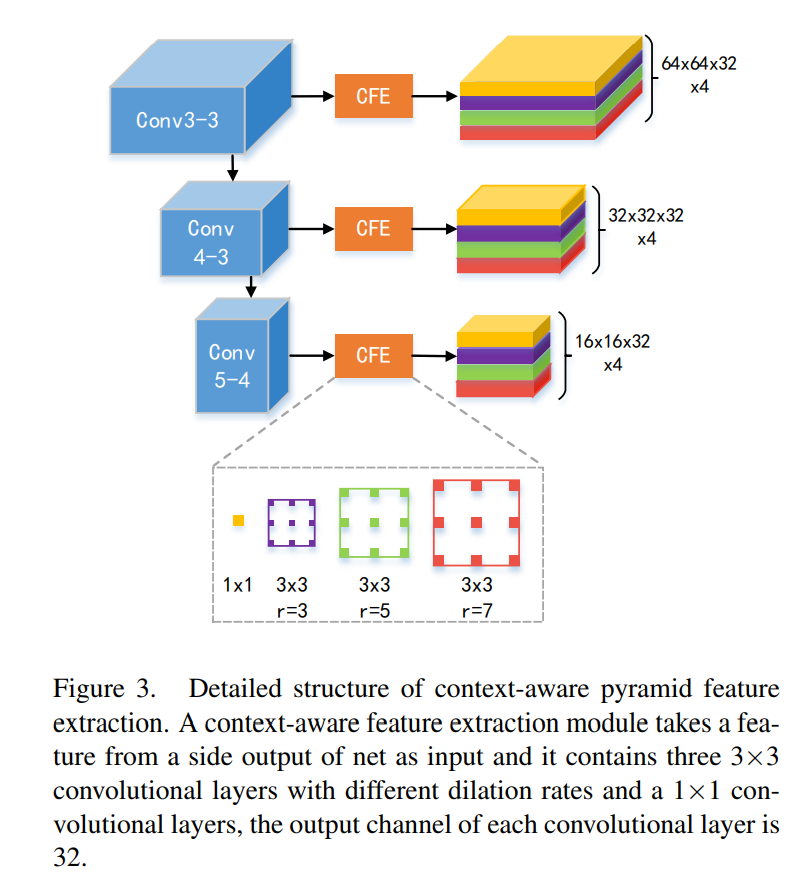
实际上就是一种ASPP结构。
class BatchNorm(BatchNormalization):def call(self, inputs, training=None):return super(self.__class__, self).call(inputs, training=True)def BN(input_tensor,block_id):bn = BatchNorm(name=block_id+'_BN')(input_tensor)a = Activation('relu',name=block_id+'_relu')(bn)return adef AtrousBlock(input_tensor, filters, rate, block_id, stride=1):x = Conv2D(filters, (3, 3), strides=(stride, stride),dilation_rate=(rate, rate),padding='same', use_bias=False,name=block_id + '_dilation')(input_tensor)return xdef CFE(input_tensor, filters, block_id):rate = [3, 5, 7]cfe0 = Conv2D(filters, (1, 1), padding='same', use_bias=False,name=block_id + '_cfe0')(input_tensor)cfe1 = AtrousBlock(input_tensor, filters, rate[0], block_id + '_cfe1')cfe2 = AtrousBlock(input_tensor, filters, rate[1], block_id + '_cfe2')cfe3 = AtrousBlock(input_tensor, filters, rate[2], block_id + '_cfe3')cfe_concat = Concatenate(name=block_id + 'concatcfe', axis=-1)([cfe0, cfe1, cfe2, cfe3])cfe_concat = BN(cfe_concat, block_id)return cfe_concat
Channel-wise attention & Spacial attention
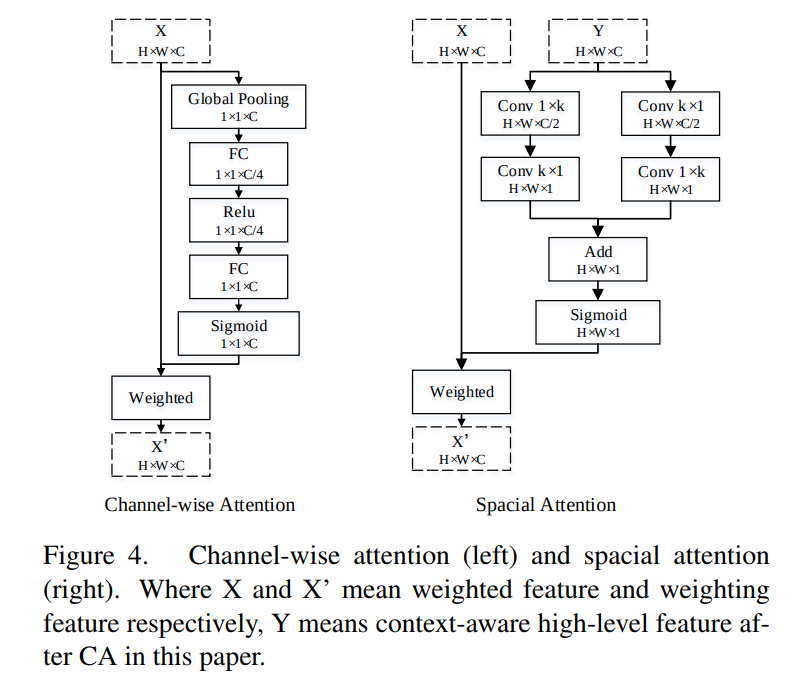
这里的通道注意力有些类似于SENet的模块,而这里的空间结构使用了非对称卷积的方式,逐步压缩通道,改变卷积方向、扩大感受野(文章中的k=9)的同时实现了较低的运算量。

两个分支加和后使用sigmoid计算得到一个权重,对原始特征加权。
import tensorflow as tffrom keras.engine import Layerfrom keras.layers import *from bilinear_upsampling import BilinearUpsamplingclass BatchNorm(BatchNormalization):def call(self, inputs, training=None):return super(self.__class__, self).call(inputs, training=True)def BN(input_tensor,block_id):bn = BatchNorm(name=block_id+'_BN')(input_tensor)a = Activation('relu',name=block_id+'_relu')(bn)return adef l1_reg(weight_matrix):return K.mean(weight_matrix)class Repeat(Layer):def __init__(self,repeat_list, **kwargs):super(Repeat, self).__init__(**kwargs)self.repeat_list = repeat_listdef call(self, inputs):outputs = tf.tile(inputs, self.repeat_list)return outputsdef get_config(self):config = {'repeat_list': self.repeat_list}base_config = super(Repeat, self).get_config()return dict(list(base_config.items()) + list(config.items()))def compute_output_shape(self, input_shape):output_shape = [None]for i in xrange(1,len(input_shape)):output_shape.append(input_shape[i]*self.repeat_list[i])return tuple(output_shape)def SpatialAttention(inputs,name):k = 9H, W, C = map(int,inputs.get_shape()[1:])attention1 = Conv2D(C / 2, (1, k), padding='same', name=name+'_1_conv1')(inputs)attention1 = BN(attention1,'attention1_1')attention1 = Conv2D(1, (k, 1), padding='same', name=name + '_1_conv2')(attention1)attention1 = BN(attention1, 'attention1_2')attention2 = Conv2D(C / 2, (k, 1), padding='same', name=name + '_2_conv1')(inputs)attention2 = BN(attention2, 'attention2_1')attention2 = Conv2D(1, (1, k), padding='same', name=name + '_2_conv2')(attention2)attention2 = BN(attention2, 'attention2_2')attention = Add(name=name+'_add')([attention1,attention2])attention = Activation('sigmoid')(attention)attention = Repeat(repeat_list=[1, 1, 1, C])(attention)return attentiondef ChannelWiseAttention(inputs,name):H, W, C = map(int, inputs.get_shape()[1:])attention = GlobalAveragePooling2D(name=name+'_GlobalAveragePooling2D')(inputs)attention = Dense(C / 4, activation='relu')(attention)attention = Dense(C, activation='sigmoid',activity_regularizer=l1_reg)(attention)attention = Reshape((1, 1, C),name=name+'_reshape')(attention)attention = Repeat(repeat_list=[1, H, W, 1],name=name+'_repeat')(attention)attention = Multiply(name=name + '_multiply')([attention, inputs])return attention
损失函数(亮点)
最终的损失函数:
其中的LS为正常的交叉熵函数,关键在于这里的LB,是一个边界损失。定义如下:
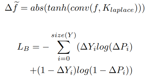
这里使用laplace算子提取边缘信息(梯度),配合 abs 和 tanh 操作得到最终的边缘,下面是相关的代码,主要差异在于 abs 改为了 relu :
import tensorflow as tffrom keras import backend as Kfrom keras.backend.common import epsilondef _to_tensor(x, dtype):return tf.convert_to_tensor(x, dtype=dtype)def logit(inputs):_epsilon = _to_tensor(epsilon(), inputs.dtype.base_dtype)inputs = tf.clip_by_value(inputs, _epsilon, 1 - _epsilon)inputs = tf.log(inputs / (1 - inputs))return inputs# 计算laplace的函数def tfLaplace(x):laplace = tf.constant([[-1, -1, -1], [-1, 8, -1], [-1, -1, -1]], tf.float32)laplace = tf.reshape(laplace, [3, 3, 1, 1])edge = tf.nn.conv2d(x, laplace, strides=[1, 1, 1, 1], padding='SAME')edge = tf.nn.relu(tf.tanh(edge))return edgedef EdgeLoss(y_true, y_pred):y_true_edge = tfLaplace(y_true)edge_pos = 2.edge_loss = K.mean(tf.nn.weighted_cross_entropy_with_logits(y_true_edge,y_pred,edge_pos), axis=-1)return edge_lossdef EdgeHoldLoss(y_true, y_pred):y_pred2 = tf.sigmoid(y_pred)y_true_edge = tfLaplace(y_true)y_pred_edge = tfLaplace(y_pred2)y_pred_edge = logit(y_pred_edge)edge_loss = K.mean(tf.nn.sigmoid_cross_entropy_with_logits(labels=y_true_edge,logits=y_pred_edge), axis=-1)saliency_pos = 1.12saliency_loss = K.mean(tf.nn.weighted_cross_entropy_with_logits(y_true,y_pred,saliency_pos), axis=-1)return 0.7*saliency_loss+0.3*edge_loss
实验细节
准备数据
- don’t use the validation set and train the model until training loss converges.
- some data augmentation techniques:
- random rotating
- random cropping
- random brightness, saturation and contrast changing
- random horizontal flipping.
下面是实验中设定的训练时的数据增强。真值与输入样本的处理略有不同,归类如下:
| Image | Mask |
|---|---|
| random_crop | random_crop |
| random_rotate | random_rotate |
| random_light | |
| Zero-center by mean pixel | y = y/y.max() |
import numpy as npimport cv2import randomdef padding(x,y):h,w,c = x.shapesize = max(h,w)paddingh = (size-h)//2paddingw = (size-w)//2temp_x = np.zeros((size,size,c))temp_y = np.zeros((size,size))temp_x[paddingh:h+paddingh,paddingw:w+paddingw,:] = xtemp_y[paddingh:h+paddingh,paddingw:w+paddingw] = yreturn temp_x,temp_ydef random_crop(x,y):h,w = y.shaperandh = np.random.randint(h/8)randw = np.random.randint(w/8)randf = np.random.randint(10)offseth = 0 if randh == 0 else np.random.randint(randh)offsetw = 0 if randw == 0 else np.random.randint(randw)p0, p1, p2, p3 = offseth,h+offseth-randh, offsetw, w+offsetw-randwif randf >= 5:x = x[::, ::-1, ::]y = y[::, ::-1]return x[p0:p1,p2:p3],y[p0:p1,p2:p3]def random_rotate(x,y):angle = np.random.randint(-25,25)h, w = y.shapecenter = (w / 2, h / 2)M = cv2.getRotationMatrix2D(center, angle, 1.0)return cv2.warpAffine(x, M, (w, h)),cv2.warpAffine(y, M, (w, h))def random_light(x):contrast = np.random.rand(1)+0.5light = np.random.randint(-20,20)x = contrast*x + lightreturn np.clip(x,0,255)def getTrainGenerator(file_path, target_size, batch_size, israndom=False):f = open(file_path, 'r')trainlist = f.readlines()f.close()while True:random.shuffle(trainlist)batch_x = []batch_y = []for name in trainlist:p = name.strip('\r\n').split(' ')img_path = p[0]mask_path = p[1]x = cv2.imread(img_path)y = cv2.imread(mask_path)x = np.array(x, dtype=np.float32)y = np.array(y, dtype=np.float32)############# 处理的核心 ######################if len(y.shape) == 3:y = y[:,:,0]y = y/y.max()if israndom:x,y = random_crop(x,y)x,y = random_rotate(x,y)x = random_light(x)x = x[..., ::-1]# Zero-center by mean pixelx[..., 0] -= 103.939x[..., 1] -= 116.779x[..., 2] -= 123.68x, y = padding(x, y)############# 处理的核心 ######################x = cv2.resize(x, target_size, interpolation=cv2.INTER_LINEAR)y = cv2.resize(y, target_size, interpolation=cv2.INTER_NEAREST)y = y.reshape((target_size[0],target_size[1],1))batch_x.append(x)batch_y.append(y)if len(batch_x) == batch_size:yield (np.array(batch_x, dtype=np.float32), np.array(batch_y, dtype=np.float32))batch_x = []batch_y = []
在测试的时候,这样设定,使用了 zero-center 、 padding 、 resize ,而预测生成的时候就要 cut 到原始的大小,再与真值计算损失(这里是猜测)。
import numpy as npimport cv2import osfrom keras.layers import Inputfrom model import VGG16import matplotlib.pyplot as pltdef padding(x):h,w,c = x.shapesize = max(h,w)paddingh = (size-h)//2paddingw = (size-w)//2temp_x = np.zeros((size,size,c))temp_x[paddingh:h+paddingh,paddingw:w+paddingw,:] = xreturn temp_xdef load_image(path):x = cv2.imread(path)sh = x.shapex = np.array(x, dtype=np.float32)# 这句似乎没什么用?x = x[..., ::-1]# Zero-center by mean pixelx[..., 0] -= 103.939x[..., 1] -= 116.779x[..., 2] -= 123.68x = padding(x)x = cv2.resize(x, target_size, interpolation=cv2.INTER_LINEAR)x = np.expand_dims(x,0)return x,shdef cut(pridict,shape):h,w,c = shapesize = max(h, w)pridict = cv2.resize(pridict, (size,size))paddingh = (size - h) // 2paddingw = (size - w) // 2return pridict[paddingh:h + paddingh, paddingw:w + paddingw]def sigmoid(x):return 1/(1 + np.exp(-x))def getres(pridict,shape):pridict = sigmoid(pridict)*255pridict = np.array(pridict, dtype=np.uint8)pridict = np.squeeze(pridict)pridict = cut(pridict, shape)return pridictdef laplace_edge(x):laplace = np.array([[-1, -1, -1], [-1, 8, -1], [-1, -1, -1]])edge = cv2.filter2D(x/255.,-1,laplace)edge = np.maximum(np.tanh(edge),0)edge = edge * 255edge = np.array(edge, dtype=np.uint8)return edgeos.environ["CUDA_DEVICE_ORDER"] = "PCI_BUS_ID"os.environ["CUDA_VISIBLE_DEVICES"] = "0"model_name = 'model/PFA_00050.h5'target_size = (256,256)dropout = Falsewith_CPFE = Truewith_CA = Truewith_SA = Trueif target_size[0 ] % 32 != 0 or target_size[1] % 32 != 0:raise ValueError('Image height and wight must be a multiple of 32')model_input = Input(shape=(target_size[0],target_size[1],3))model = VGG16(model_input,dropout=dropout, with_CPFE=with_CPFE, with_CA=with_CA, with_SA=with_SA)model.load_weights(model_name,by_name=True)for layer in model.layers:layer.trainable = Falseimage_path = 'image/2.jpg'img, shape = load_image(image_path)img = np.array(img, dtype=np.float32)sa = model.predict(img)sa = getres(sa, shape)edge = laplace_edge(sa)...
训练
- When training, we set α = 1.0 at beginning to generate rough saliency map. In this period, our model is trained using SGD with an initial learning rate 1e-2, the image size is 256×256 , the batch size is 22.
- Then we adjust different α to refine the boundaries of saliency map,and find α = 0.7 is the optimal setting in experiment Tab.2. In this period, the image size, batch size is same as the previous period, but the initial learning rate is 1e-3.
这里的 alpha 就是两个损失之间的权重比例。
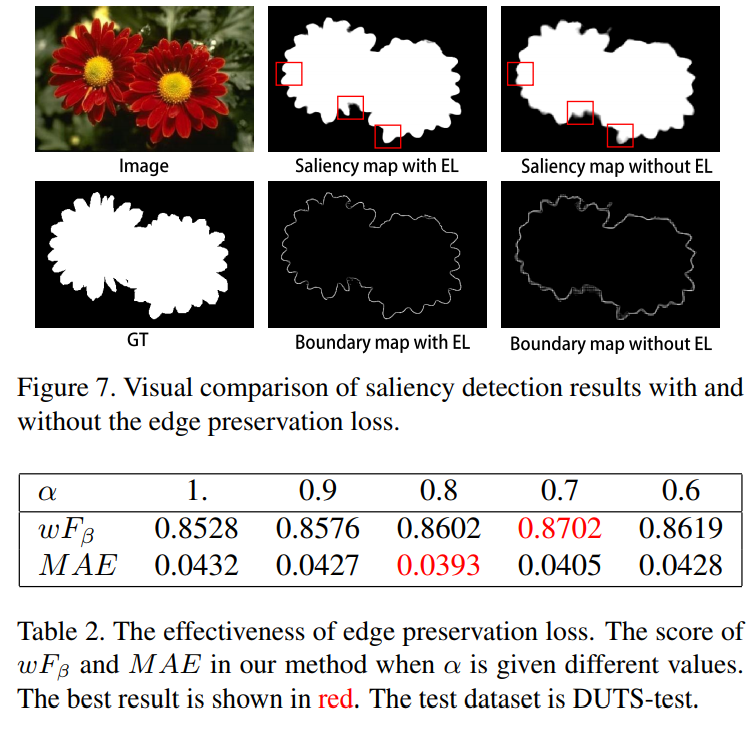
从上图中可以看出来,添加边界保留损失的时候,确实一定程度上得到较为清晰的边界。
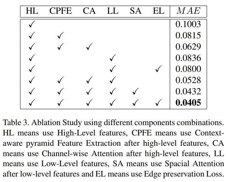
消融实验
参考链接

若有收获,就点个赞吧
0 人点赞
