SegFix: Model-Agnostic Boundary Refinement for Segmentation

说在开头

后处理算法

本文提出了一种后处理算法，想要对标DenseCRF[Efficient inference in fully connected crfs with gaussian
edge potentials]，最终实现了超越DenseCRF的性能。不过可惜的是，这里没有与DenseCRF进行速度上的比较，毕竟，DenseCRF的痛点还是在于速度。
不知道这里会不会也有这样的问题，如果速度和精度都会高于DenseCRF的话，那就真的很棒了。当然这里的讨论前提是，对于一副测试图像而言，不会进行事先的处理，而是在使用的时候即时处理。之所以这么说，是因为本文的方法可以通过事先生成测试数据的边缘图和方向图（实际在文章中也是这么做的），直接用其来调整现有模型生成的预测在边缘附近的预测，从而节省一些使用该方案后处理的时间。DenseCRF是完全依赖于网络的预测的，所以说它的耗时是实打实的累加在推理时间上的。

边缘信息

这里的后处理的出发点也很直接，考虑到了分割任务中的难样本的处理，即边缘附近像素的预测结果的优化。边缘附近的预测是大多数深度学习分割方法的共有的痛点之一。文章也简单统计了几个主流模型的误差像素的位置分布：

从图中可以看到，预测误差的主要来源就是边界附近的区域。所以论文也会提到： Our work is mainly motivated by the observation that most of the existing state-of-the-art segmentation models fail to deal well with the error predictions along the boundary.
所以也有很多方法在尝试解决这个问题，一些方法会引入边界信息来提升分割效果，甚至是引入边缘检测任务以多任务学习的形式来强化边缘的预测。但是这些方法与模型整体集成过于紧密，并不能像DenseCRF那样作为单独的后处理，来实现对于现有方法的普遍增强。

核心思路

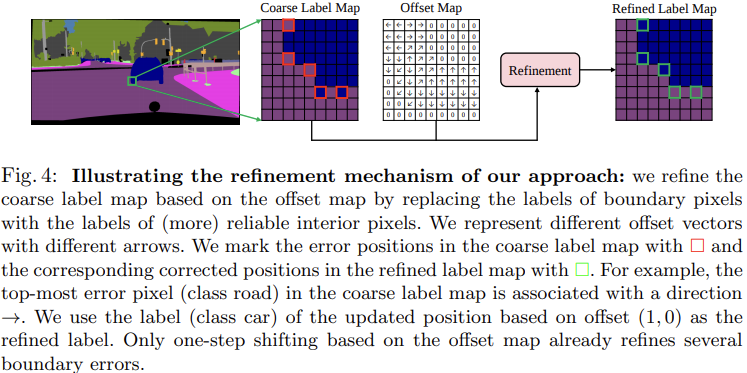
本文的方法概括起来很简单，就是让边缘区域的像素的预测结果，直接使用其相同类别区域内部像素的预测（因为区域内部的预测一般都很准确）。
所以首要的问题在于：

1. 如何确定边缘像素？
2. 如何关联边缘像素与内部像素？

这里主要借助于一个边缘预测分支和一个方向预测分支来完成。
在获得良好的边界和方向预测之后，就可以直接拿来优化现有方法预测的分割图了。所以另一个问题在于，如何将现有的针对边缘的关联方向的预测应用到实际的预测优化上。
这主要借助于一个坐标偏移分支。

The key condition for ensuring the effectiveness of our approach is that segmentation predictions of the interior pixels are more reliable empirically. Given accurate boundary maps and direction maps, we could always improve the segmentation performance in expectation. In other words, the segmentation performance ceiling of our approach is also determined by the interior pixels’ prediction accuracy.

主体结构

主要包含两块内容，一部分是通过数据事先训练得到的用来生成边缘区域坐标偏移图的结构，一部分是通过使用偏移图来优化现有模型在边缘区域上的预测的结构。
Considering that there might be some “fake” interior pixels when the boundary is thick, we propose two different schemes as following:

1. re-scaling all the offsets by a factor, e.g., 2.
2. iteratively applying the offsets (of the “fake” interior pixels) until finding an interior pixel.

We choose (1) by default for simplicity as their performance is close.

We use ”fake” interior pixels to represent pixels (after offsets) that still lie on the boundary when the boundary is thick. Notably, we identify an pixel as interior pixel/boundary pixel if its value in the predicted boundary map B is 0/1.

边缘预测分支

• 1×1 Conv -> BN -> ReLU with 256 output channels -> a linear classifier (1x1 Conv) -> Up-sample the prediction to genereate the final boundary map which records the probability of the pixel belonging to the boundary
• 训练时由真值boundary map监督约束，使用二值交叉熵损失作为边界损失，学习良好的边缘检测

• 测试时直接生成边缘图

  方向预测分支

• 1 × 1 Conv -> BN -> ReLU with 256 output channels -> a linear classifier (1×1 Conv) -> Up-sample the classifier prediction to generate the final direction map . We mask the direction map by multiplying by the (binarized) boundary map to ensure that we only apply direction loss on the pixels identified as boundary by the boundary branch.

• 预测所有位置的像素与之最近的同类像素的方向，这里的方向不是连续的，而是对量化成m个值后的结果（In fact, we empirically find that our discrete categorization scheme outperforms the regression scheme, e.g., mean squared loss in the angular domain [Deep watershed transform for instance segmentation], measured by the final segmentation performance improvements）
• 训练时使用真值direction map监督该分支生成的离散方向，使用多分类交叉熵损失（standard category-wise cross-entropy loss）来作为方向预测损失

• 测试时同样直接生成离散方向图

  获取真值

  

• 都由分割任务的mask来生成（语义分割、实例分割都是如此）

• 需要先生成distance map，再在此基础上生成boundary map和direction map
  • 对于每个像素而言，distance map上都记录了它相距于属于其他类别像素的最小欧式距离。这实际上也表示了像素到边界的距离
  • 首先将真值mask分解成K个binary map (0 or 1)，每个map关联着不同的类别（语义类别、实例类别），K表示图像中包含的类别数量。之后在每个binary map上独立计算distance map，这里使用了scipy的函数scipy.ndimage.morphology.distance_transform_edt() ，这个函数用于距离转换，计算图像中非零点到最近背景点（即0）的距离。它被用在每个类别独立的binary mask上，正好计算的就是相距于其他类别（每个binary mask上的0表示的就是“其他类别”）的最小欧氏距离
  • 计算完各个mask之后，我们可以计算一个融合的distance map来实现对于所有的K个distance map的集成
• boundary map
  • 使用融合后的distance map，对其使用一个预设的阈值进行划分，小于阈值的作为边界区域的像素，大于阈值的认为在特定目标区域内部。因为距离值越小，说明越接近边界

• direction map（如图5中的示例）

  • 这里在未合并的K层distance map上，分别使用9x9的Sobel滤波器。基于Sobel滤波器的方向是在内，并且每个像素位置的方向都指向邻域内部距离目标边界最远的像素
  • 整个方向范围被均匀划分（量化）成了m类，然后每个像素的方向被赋值成对应的方向类别 :::info 让人疑惑的是，这里是如何通过Sobel算子获得方向图的？论文中对此并没有太详细的解释

• 关于大核Sobel算子的计算方式：https://stackoverflow.com/questions/9567882/sobel-filter-kernel-of-large-size :::

  坐标偏移分支

  

• 用来转换预测得到的（已经乘过了）到坐标偏移图

• 不同的方向会被映射到不同的坐标偏移值，例如图5(a)中所示，对于m=4的右上方向，可以映射为(1, 1)
• 最终通过坐标映射（the grid-sample scheme [Spatial transformer networks]），重新对现有方法在边界区域的预测结果进行调整，图4中给出了一个例子

• 使用调整现有粗糙预测的公式为：，即将每个位置上最终的预测，设定为坐标偏移后对应位置的原始预测结果

  重要实验结果

  
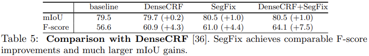
  我比较关注这个实验。该方法与DenseCRF并不冲突，效果很不错。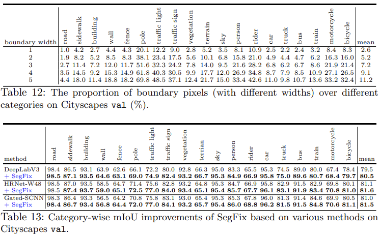
  
  另外这个实验也说明了，对于边缘区域占比较大的目标，效果提升更加明显，这一点也是可以理解的，因为这个方法重点在于优化边缘。

  相关链接

• 论文：https://arxiv.org/pdf/2007.04269.pdf

• 代码：https://github.com/openseg-group/openseg.pytorch