图片 - Cascaded Partial Decoder for Fast and Accurate Salient Object Detection - 《深度学习论文阅读》

几个亮点
网络结构
- 双分支
- 训练
整体注意力模块(Holistic Attention Module)
解码器
实验细节
总结
启发
参考代码

几个亮点

速度快：
1. 后续计算只利用了编码器的后三个卷积块的输出特征，没有使用前两个，因为前两个尺寸比较大，计算消耗比较大，这个是大头，与初始注意力图相比，所提出的整体注意机制几乎不会增加计算成本，并进一步突出了整个显着对象，如图4所示。
2. 为了加速，在每个分支都是用1x1卷积将通道降维到32，并使用了Skip连接。
精度高：
1. 结构的有效性。双分支结构，一路生成初始显著性图，一路生成更高质量的显著性图，前者用来细化后者的特征信息，抑制干扰信息。
2. 使用整体注意力模块(holistic attention module)，扩大初始显着图的覆盖范围。
3. decoder中使用改进的RFB模块，多尺度感受野，有效编码上下文
4. 两个分支中都使用了多尺度的特征，来自不同的层级。

网络结构

Cascaded Partial Decoder for Fast and Accurate Salient Object Detection - 图2

现有的优秀的显著性目标检测网络主要依赖于集成来自预训练网络的多级特征，但是相比高级特征：

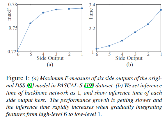
低级特征实际上对于深度集成模型的性能贡献较少（下图a）
低级特征集成到高级特征上，会增大计算消耗，因为它们空间分辨率比较大（下图b）

下图比较了原始的DSS模型在Pascal-S数据集六个输出的maxF的值，并且也计算了六个输出的推理时间。可以看出，最靠前的特征对于性能的增益减小，而其推理时间却增长的很大

另外文章的结果也反映出来，仅仅集成后面的特征也可以获得相对准确的结果。于是这里设计的结构就去掉了过于浅层的特征，从第三层开始使用。但是为什么要从第三层开始呢？下面简单解释了下。

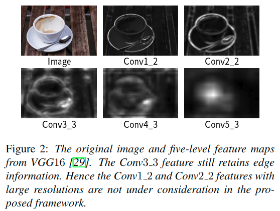
随着网络加深，特征逐渐从低级表示演化为高级表示。因此，当仅集成更深层的特征时，深度聚合模型可以恢复显着性图的空间细节。在图2中，展示了VGG16的多级特征图的例子。与Conv1_2和Conv2_2的低级特征相比，Conv3_3的特征也保留了边缘信息。

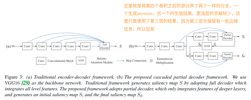
使用这里作为优optimization layer，使用后两个卷积块来构造双分支（注意力分支与检测分支）。

双分支

设计partial decoder集成来自三个卷积块的输出特征（f3，f4，f5），进而得到初始显著性图Si。
经过整体注意力模块的处理之后，得到增强的注意力图Sh，用其细化来自第三个卷积块的特征f3。因为这里可以通过聚合三个顶层的特征来获得一个相对精确的显著性图，这里的注意力图就可以有效的消除特征f3中的异常信息，并且极大的提升其表达能力。
- 如果将干扰归为显着性部分，则该策略导致异常分割结果。因此，需要提高初始显着性图的有效性。使用了整体注意力模块
通过特征图f3与注意力图Sh的元素乘法可以获得细化的特征图f3d，进过卷积4和5可以得到对应的输出f4d和f5d。
细化后的特征最终通过另一个partial decoder得到输出的显著性图Sd。

此外，提出的框架可用于改进现有的深度聚合模型。在提出的框架中嵌入解码器时，准确性和效率将得到显着提高。

训练

两个分支使用真值联合训练，Si和Sd分别与真值计算交叉熵并求和，进而得到整体的损失。

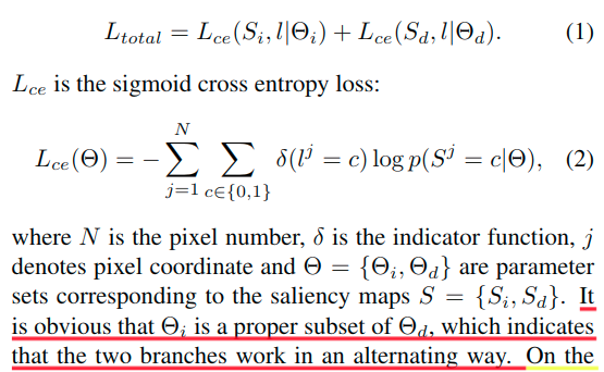
很明显，Thetai是Thetad的的适当子集，这表明两个分支以交替的方式工作。

一方面，注意力分支为检测分支提供精确的注意图，这导致检测分支更精确的显着对象。
另一方面，检测分支可以被认为是注意力分支的辅助损失，这也有助于注意力分支集中于显着对象。

联合训练两个分支使模型统一突出显着的物体，同时抑制干扰物。

此外，可以利用提出的框架来改进现有的深度聚合模型，通过使用这些工作的聚合算法来整合每个分支的特征。

尽管与传统的编码器 - 解码器架构相比，这里增加了一个解码器提高了骨干网络的计算成本，但由于丢弃了解码器中的低级特征，总计算复杂度仍然显着降低。此外，所提出的框架的级联优化机制提升了性能，实验表明这两个分支都优于原始模型。

整体注意力模块(Holistic Attention Module)

给定来自优化层（Conv3_3）的特征映射和来自注意力分支的初始显着性图，可以使用初始注意力策略，这意味着直接将特征映射与初始显着性图相乘。

当从注意力分支获得准确的显着性图时，该策略将有效地抑制特征的干扰。
相反，如果将干扰归类为显着性区域，则该策略导致异常分割结果。

因此，需要提高初始显着性图的有效性。更具体地说，显着性目标的边缘信息可能被初始显着性图过滤掉，因为难以精确预测。另外，复杂场景中的一些对象很难被完全分割。因此提出了一个整体注意力模块，来扩大初始显著性图的覆盖范围。

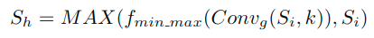
这里的Convg表示一个有着高斯核k和零偏置的卷积操作，其中的fmin_max()表示一个归一化函数，来让blurred map的范围变为[0, 1]。而MAX()操作表示取最大值函数，这样可以使得趋向于增加平滑后的Si中显著性区域的权重系数。

相较于初始的注意力，提出的整体注意力机制增加了一定的计算消耗，但是也进一步高亮了整体显著性目标。

注意，这里的高斯核k的尺寸和标准差被初始化为32和4，在训练中会自动学习。

解码器

由于框架由两个解码器组成，需要构建一个快速集成策略以确保低复杂性。同时，需要尽可能准确地生成显着图。

在解码器中使用了改进的RFB(receptive field block)模块
- 本身的RFB是将Inception模块中的3x3卷积替换为扩张卷积
- 在RFB上也使用了Skip连接
- 这样可以实现多尺度的感受野，进一步捕获全局对比度信息，更加有效的编码上下文信息
为了加速，在每个分支都用1x1卷积降低通道为32。

这里对于特征聚合有如下公式：

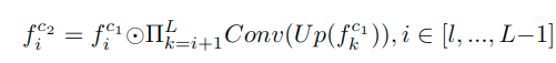
但是不够直观，可以看代码：

class CPD_ResNet(nn.Module):
    # resnet based encoder decoder
    def __init__(self, channel=32):
        super(CPD_ResNet, self).__init__()
        self.resnet = B2_ResNet()
        self.rfb2_1 = RFB(512, channel)
        self.rfb3_1 = RFB(1024, channel)
        self.rfb4_1 = RFB(2048, channel)
        self.agg1 = aggregation(channel)
        self.rfb2_2 = RFB(512, channel)
        self.rfb3_2 = RFB(1024, channel)
        self.rfb4_2 = RFB(2048, channel)
        self.agg2 = aggregation(channel)
        self.upsample = nn.Upsample(scale_factor=8, mode='bilinear', align_corners=True)
        ...
    def forward(self, x):
        ...
        x2_1 = x2
        x3_1 = self.resnet.layer3_1(x2_1)  # 1024 x 16 x 16
        x4_1 = self.resnet.layer4_1(x3_1)  # 2048 x 8 x 8
        x2_1 = self.rfb2_1(x2_1)
        x3_1 = self.rfb3_1(x3_1)
        x4_1 = self.rfb4_1(x4_1)
        attention_map = self.agg1(x4_1, x3_1, x2_1)
        x2_2 = self.HA(attention_map.sigmoid(), x2)
        x3_2 = self.resnet.layer3_2(x2_2)  # 1024 x 16 x 16
        x4_2 = self.resnet.layer4_2(x3_2)  # 2048 x 8 x 8
        x2_2 = self.rfb2_2(x2_2)
        x3_2 = self.rfb3_2(x3_2)
        x4_2 = self.rfb4_2(x4_2)
        detection_map = self.agg2(x4_2, x3_2, x2_2)
        return self.upsample(attention_map), self.upsample(detection_map)

代码中使用了RFB模块，具体代码可见最后。它的作用就是多尺度感受野，上下文信息的编码，也起到了降维的作用，输出都是32通道，对于每个前面模块的特征都会进行一下处理，这里用在了f3,f4,f5和f3d,f4d,f5d上。关键在于这里的特征聚合模块。

class aggregation(nn.Module):
    # dense aggregation, it can be replaced by other aggregation model, such as DSS, amulet, and so on.
    # used after MSF
    def __init__(self, channel):
        super(aggregation, self).__init__()
        self.relu = nn.ReLU(True)
        self.upsample = nn.Upsample(scale_factor=2, mode='bilinear', align_corners=True)
        self.conv_upsample1 = BasicConv2d(channel, channel, 3, padding=1)
        self.conv_upsample2 = BasicConv2d(channel, channel, 3, padding=1)
        self.conv_upsample3 = BasicConv2d(channel, channel, 3, padding=1)
        self.conv_upsample4 = BasicConv2d(channel, channel, 3, padding=1)
        self.conv_upsample5 = BasicConv2d(2*channel, 2*channel, 3, padding=1)
        self.conv_concat2 = BasicConv2d(2*channel, 2*channel, 3, padding=1)
        self.conv_concat3 = BasicConv2d(3*channel, 3*channel, 3, padding=1)
        self.conv4 = BasicConv2d(3*channel, 3*channel, 3, padding=1)
        self.conv5 = nn.Conv2d(3*channel, 1, 1)
    def forward(self, x1, x2, x3):
        x1_1 = x1
        x2_1 = self.conv_upsample1(self.upsample(x1)) * x2
        x3_1 = self.conv_upsample2(self.upsample(self.upsample(x1))) \
               * self.conv_upsample3(self.upsample(x2)) * x3
        x2_2 = torch.cat((x2_1, self.conv_upsample4(self.upsample(x1_1))), 1)
        x2_2 = self.conv_concat2(x2_2)
        x3_2 = torch.cat((x3_1, self.conv_upsample5(self.upsample(x2_2))), 1)
        x3_2 = self.conv_concat3(x3_2)
        x = self.conv4(x3_2)
        # N,96,H//8,W//8
        x = self.conv5(x)
        return x

按照代码注释，可以看出，这里是可以被替换的，可以替换为其他的网络的聚合模块。注意这里在进行聚合的时候，使用的是乘法的操作。上采样到相同尺度之后经过卷积的特征与对应尺度的另一个输入特征进行乘法操作。下面简单绘制了一下这个流程：

Cascaded Partial Decoder for Fast and Accurate Salient Object Detection - 图8 这里最后输出的特征图还需要双线性插值上采样8倍。最终使用1x1卷积进行预测输出。

实验细节

Pytorch framework and a GTX 1080Ti GPU
Train：DUTS-TR
The parameters of the bifurcated backbone network are initialized by VGG16.
We initialize the other convolutional layers using the default setting of the Pytorch.
All training and test images are resized to 352x352.
Any post-processing procedure (e.g. CRF) is not applied in this paper.
The proposed model is trained by Adam optimizer. The batch size is set as 10 and the initial learning rate is set as 1e-4 and decreased by 10% when training loss reaches a flat.
It takes nearly six hours for training the proposed model.

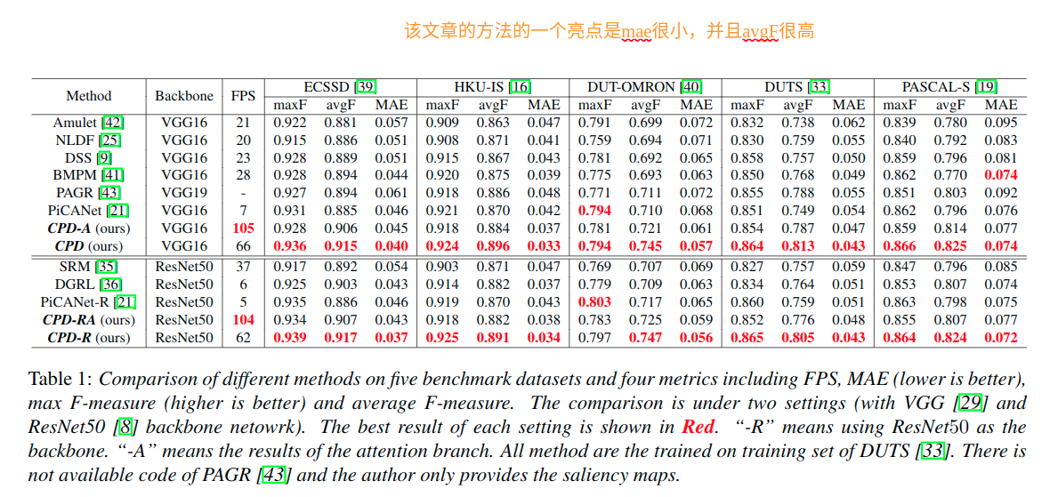
提出的模型在avgF得分方面比MAE和maxF得到更多改善。这种现象是由于所提出的联合训练策略。

一方面，注意力分支的被监督的注意力图使得检测分支进一步集中于显着对象。
另一方面，当训练所提出的模型时，检测分支的梯度也向后传播到注意力分支。

该训练机制逐渐促进所提出的模型专注于显着对象。

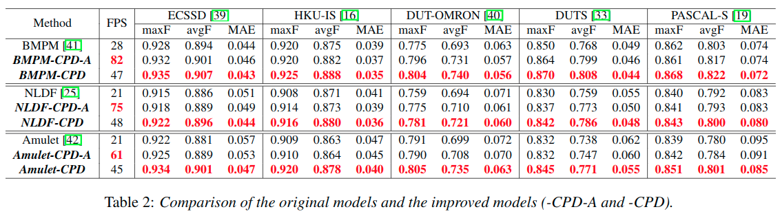
使用CPD结构来提升现有的BMPM和NLDF以及Amulet结构，效果如下。不论速度还是精度都有提升。

NLDF adopts a typical U-Net architecture, BMPM proposes a bidirectional decoder with gate function and Amulet integrates multi-level feature maps in multiple resolutions.

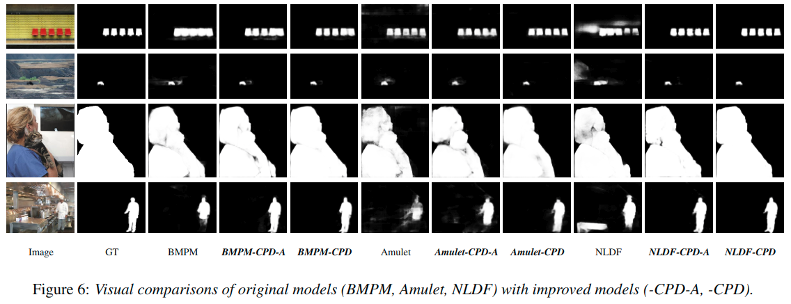
在图6中，展示了较难的案例的量化结果：多个目标，小目标，大目标和复杂场景。上面两行显示改进的模型进一步关注目标区域并抑制干扰。两行以下显示

holistic attention的有效性

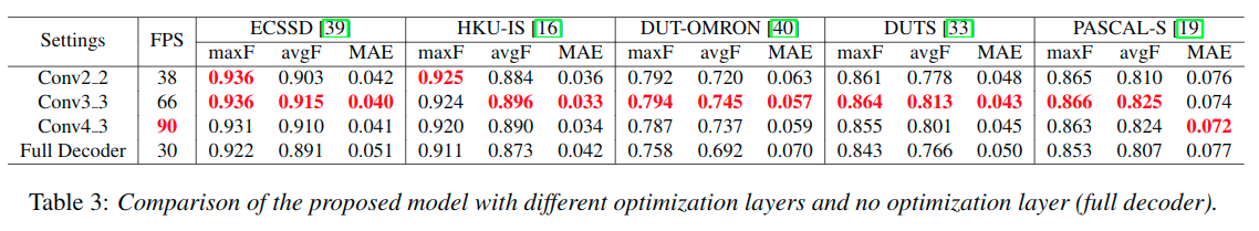
optimization layer的选择

We do not test the proposed model with Conv12 optimization layer because this setting will increase the computation cost via adding one more full decoder; thus requirements of reducing computation cost will not be achieved.

失败案例

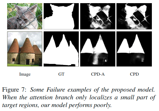
The performance of the proposed model relies on the accuracy of the attention branch. When the attention branch detects clutters as target regions, our model will obtain wrong results.

其他应用

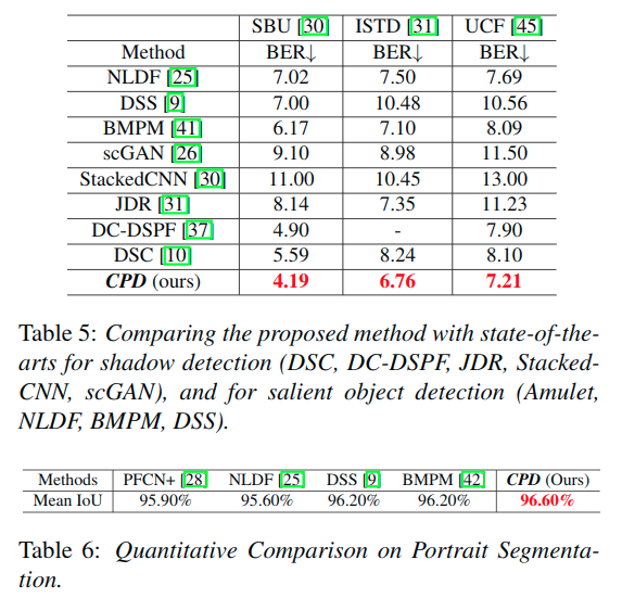
也在阴影检测和肖像分割的任务中进行了训练测试，得到了不错的效果。

总结

本文提出了一种新颖的级联部分解码器框架，用于快速准确的显着物体检测。
在构造解码器时，所提出的框架丢弃较浅层的特征以提高计算效率，并利用生成的显着图来细化特征以提高准确性。
提出了一个整体注意模块来进一步细分整个显着对象
提出一个有效的解码器来抽象判别特征并快速整合多层次特征

实验表明，模型在五个基准数据集上实现了最先进的性能，并且比现有的深度模型运行得更快。为了证明所提出的框架的一般化，将其应用于改进现有的深度聚合模型并显着提高其准确性和效率。此外，验证了所提出的模型在阴影检测和肖像分割两个任务中的有效性。

启发

有效的分割不见得需要利用所有的层级
对于需要细化的特征使用注意力机制
对注意力分支也进行真值的监督
扩大感受野的同时尽可能减少计算量（使用扩张Inception模块的扩张卷积改进，并配合skip链接）
测试在其他相似任务上的有效性

参考代码

https://github.com/wuzhe71/CPD

# https://github.com/wuzhe71/CPD/blob/master/model/CPD_ResNet_models.py
import torch
import torch.nn as nn
import torchvision.models as models
from HolisticAttention import HA
from ResNet import B2_ResNet
class BasicConv2d(nn.Module):
    def __init__(self, in_planes, out_planes, kernel_size, stride=1, padding=0, dilation=1):
        super(BasicConv2d, self).__init__()
        self.conv = nn.Conv2d(in_planes, out_planes,
                              kernel_size=kernel_size, stride=stride,
                              padding=padding, dilation=dilation, bias=False)
        self.bn = nn.BatchNorm2d(out_planes)
        self.relu = nn.ReLU(inplace=True)
    def forward(self, x):
        x = self.conv(x)
        x = self.bn(x)
        return x
class RFB(nn.Module):
    # RFB-like multi-scale module
    def __init__(self, in_channel, out_channel):
        super(RFB, self).__init__()
        self.relu = nn.ReLU(True)
        self.branch0 = nn.Sequential(
            BasicConv2d(in_channel, out_channel, 1),
        )
        self.branch1 = nn.Sequential(
            BasicConv2d(in_channel, out_channel, 1),
            BasicConv2d(out_channel, out_channel, kernel_size=(1, 3), padding=(0, 1)),
            BasicConv2d(out_channel, out_channel, kernel_size=(3, 1), padding=(1, 0)),
            BasicConv2d(out_channel, out_channel, 3, padding=3, dilation=3)
        )
        self.branch2 = nn.Sequential(
            BasicConv2d(in_channel, out_channel, 1),
            BasicConv2d(out_channel, out_channel, kernel_size=(1, 5), padding=(0, 2)),
            BasicConv2d(out_channel, out_channel, kernel_size=(5, 1), padding=(2, 0)),
            BasicConv2d(out_channel, out_channel, 3, padding=5, dilation=5)
        )
        self.branch3 = nn.Sequential(
            BasicConv2d(in_channel, out_channel, 1),
            BasicConv2d(out_channel, out_channel, kernel_size=(1, 7), padding=(0, 3)),
            BasicConv2d(out_channel, out_channel, kernel_size=(7, 1), padding=(3, 0)),
            BasicConv2d(out_channel, out_channel, 3, padding=7, dilation=7)
        )
        self.conv_cat = BasicConv2d(4*out_channel, out_channel, 3, padding=1)
        self.conv_res = BasicConv2d(in_channel, out_channel, 1)
    def forward(self, x):
        x0 = self.branch0(x)
        x1 = self.branch1(x)
        x2 = self.branch2(x)
        x3 = self.branch3(x)
        x_cat = self.conv_cat(torch.cat((x0, x1, x2, x3), 1))
        x = self.relu(x_cat + self.conv_res(x))
        return x
class aggregation(nn.Module):
    # dense aggregation, it can be replaced by other aggregation model, such as DSS, amulet, and so on.
    # used after MSF
    def __init__(self, channel):
        super(aggregation, self).__init__()
        self.relu = nn.ReLU(True)
        self.upsample = nn.Upsample(scale_factor=2, mode='bilinear', align_corners=True)
        self.conv_upsample1 = BasicConv2d(channel, channel, 3, padding=1)
        self.conv_upsample2 = BasicConv2d(channel, channel, 3, padding=1)
        self.conv_upsample3 = BasicConv2d(channel, channel, 3, padding=1)
        self.conv_upsample4 = BasicConv2d(channel, channel, 3, padding=1)
        self.conv_upsample5 = BasicConv2d(2*channel, 2*channel, 3, padding=1)
        self.conv_concat2 = BasicConv2d(2*channel, 2*channel, 3, padding=1)
        self.conv_concat3 = BasicConv2d(3*channel, 3*channel, 3, padding=1)
        self.conv4 = BasicConv2d(3*channel, 3*channel, 3, padding=1)
        self.conv5 = nn.Conv2d(3*channel, 1, 1)
    def forward(self, x1, x2, x3):
        x1_1 = x1
        x2_1 = self.conv_upsample1(self.upsample(x1)) * x2
        x3_1 = self.conv_upsample2(self.upsample(self.upsample(x1))) \
               * self.conv_upsample3(self.upsample(x2)) * x3
        x2_2 = torch.cat((x2_1, self.conv_upsample4(self.upsample(x1_1))), 1)
        x2_2 = self.conv_concat2(x2_2)
        x3_2 = torch.cat((x3_1, self.conv_upsample5(self.upsample(x2_2))), 1)
        x3_2 = self.conv_concat3(x3_2)
        x = self.conv4(x3_2)
        x = self.conv5(x)
        return x
class CPD_ResNet(nn.Module):
    # resnet based encoder decoder
    def __init__(self, channel=32):
        super(CPD_ResNet, self).__init__()
        self.resnet = B2_ResNet()
        self.rfb2_1 = RFB(512, channel)
        self.rfb3_1 = RFB(1024, channel)
        self.rfb4_1 = RFB(2048, channel)
        self.agg1 = aggregation(channel)
        self.rfb2_2 = RFB(512, channel)
        self.rfb3_2 = RFB(1024, channel)
        self.rfb4_2 = RFB(2048, channel)
        self.agg2 = aggregation(channel)
        self.upsample = nn.Upsample(scale_factor=8, mode='bilinear', align_corners=True)
        self.HA = HA()
        if self.training:
            self.initialize_weights()
    def forward(self, x):
        x = self.resnet.conv1(x)
        x = self.resnet.bn1(x)
        x = self.resnet.relu(x)
        x = self.resnet.maxpool(x)
        x1 = self.resnet.layer1(x)  # 256 x 64 x 64
        x2 = self.resnet.layer2(x1)  # 512 x 32 x 32
        x2_1 = x2
        x3_1 = self.resnet.layer3_1(x2_1)  # 1024 x 16 x 16
        x4_1 = self.resnet.layer4_1(x3_1)  # 2048 x 8 x 8
        x2_1 = self.rfb2_1(x2_1)
        x3_1 = self.rfb3_1(x3_1)
        x4_1 = self.rfb4_1(x4_1)
        attention_map = self.agg1(x4_1, x3_1, x2_1)
        x2_2 = self.HA(attention_map.sigmoid(), x2)
        x3_2 = self.resnet.layer3_2(x2_2)  # 1024 x 16 x 16
        x4_2 = self.resnet.layer4_2(x3_2)  # 2048 x 8 x 8
        x2_2 = self.rfb2_2(x2_2)
        x3_2 = self.rfb3_2(x3_2)
        x4_2 = self.rfb4_2(x4_2)
        detection_map = self.agg2(x4_2, x3_2, x2_2)
        return self.upsample(attention_map), self.upsample(detection_map)
    def initialize_weights(self):
        res50 = models.resnet50(pretrained=True)
        pretrained_dict = res50.state_dict()
        all_params = {}
        for k, v in self.resnet.state_dict().items():
            if k in pretrained_dict.keys():
                v = pretrained_dict[k]
                all_params[k] = v
            elif '_1' in k:
                name = k.split('_1')[0] + k.split('_1')[1]
                v = pretrained_dict[name]
                all_params[k] = v
            elif '_2' in k:
                name = k.split('_2')[0] + k.split('_2')[1]
                v = pretrained_dict[name]
                all_params[k] = v
        assert len(all_params.keys()) == len(self.resnet.state_dict().keys())
        self.resnet.load_state_dict(all_params)