Context Encoding for Semantic Segmentation

最近的工作通过采用Dilated / Atrous卷积, 利用多尺度特征和改进边界，在利用完全卷积网络（FCN）框架改进像素标注的空间分辨率方面取得了重大进展。

在本文中，我们通过引入上下文编码模块来探索全局上下文信息在语义分割中的影响，上下文编码模块捕获场景的语义上下文并选择性地高亮依赖于类的特征图。所提出的上下文编码模块显着改善了语义分割结果，在FCN之上只产生了一点点的额外计算成本。

本文提出了上下文编码模块(Context Encoding Module)引入全局上下文信息(global contextual information)，用于捕获场景的上下文语义并选择性的突出与类别相关的特征图。 并结合现先进的扩张卷积策略和多尺度策略提出了语义分割框架EncNet(Context Encoding Network)。

实验证明上下文编码模块能够显著的提升语义分割性能，在Pascal-Context上达到了51.7%mIoU, 在 PASCAL VOC 2012上达到了85.9% mIoU，单模型在ADE20K测试集上达到了0.5567。 此外,论文进一步讨论上下文编码模块在相对浅层的网络中提升特征表示的能力，在CIFAR-10数据集上基于14层的网络达到了3.45%的错误率，和比这个多10倍的层网络有相当的表现。

扩张卷积存在的问题

先进的语义分割系统通常是基于FCN架构，采用的深度卷积神经网络受益于从不同图片中学习到的丰富的对象类别信息和场景语义。CNN通过堆叠带非线性激活和下采样的卷积层能够捕获带全局接受野的信息表示，为了克服下采样带来的空间分辨率损失，最近的工作使用扩张卷积策略从预训练模型上产生密集预测。然而，此策略依然会将像素从全局场景上下文相隔开，这会导致像素错误分类。

金字塔结构存在的问题

近期的工作使用基于金字塔多分辨率表示扩大接受野。例如:

• PSPNet采用的PSP模块将特征图池化为不同尺寸，再做联接上采样；
• DeepLab采用ASPP模块并行的使用大扩张率卷积扩大接受野。

这些方法都有提升，但是这对上下文表示都不够明确，这出现了一个问题：捕获上下文信息是否等同于增加接受野大小？

如果我们能够先捕获到图像上下文信息(例如这是卧室)，然后，这可以提供许多相关小型目标的信息(例如卧室里面有床、椅子等)。这可以动态的减少搜索区域可能。说白了，这就是加入一个场景的先验知识，这样对图片中像素分类更有目的性。

依照这个思路，可以设计一种方法，充分利用场景上下文和存在类别概率的之间的强相关性，这样语义分割会就容易很多。

通过传统图像方法引入图像全局上下文信息

经典的计算机视觉方法具有捕获场景上下文语义的优点。例如:

• SIFT提取密集特征或滤波器组响应密集提取图像特征.
• BoW，VLAD和Fish Vector通过类别编码描述特征统计信息, 学习一个视觉字典。

经典表示通过捕获特征统计信息编码全局信息，虽然手工提取特征通过CNN方法得到了很大的改进，但传统方法的总体编码过程更为方便和强大。

我们能否利用经典方法的上下文编码结合深度学习？

最近的工作在CNN框架中传统编码器的泛化化方面取得了很大进展.

Zhang等人引入了一个编码层，它将整个字典学习和残差编码管道集成到一个CNN层中，以捕获无序表示。这种方法有在纹理分类方面取得了最先进的成果。在这项工作中，我们扩展编码层捕获全局特征统计信息以理解语义上下文。

贡献

主要详细来说是三个贡献：

1. 引入上下文编码模块，用于捕获全局尝尽上下文信息，和选择性的突出类别相关的特征图。
2. 提出了一个语义编码损失（Semantic Encoding Loss， SE-Loss），可以进一步在训练中强调场景的全局信息，使得网络能够预测场景中对象类别的存在，强化网络学习上下文语义信息。与逐像素的损失不同，SE-Loss对于大小不同的物体有相同的贡献，在实践中这能够改善识别小物体的表现，这里提出的上下文编码模块和语义编码损失在概念上是直接的并且和现存的FCN方法是兼容的。
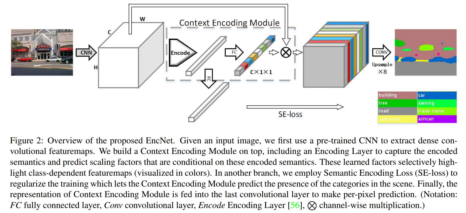
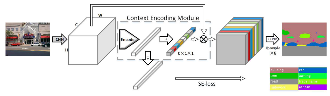
3. 设计了一个新的语义分割架构Context Encoding Network（EncNet），如前图所示，EncNet通过上下文编码模块增强了预训练的ResNet。

Context Encoding

对于预训练网络，使用编码层捕获特征图的统计信息作为全局上下文语义，将编码层的输出作为编码语义(encoded semantics)，为了使用上下文，预测了一组放缩因子(scaling factors)用于突出和类别相关的特征图。编码层学习带有上下文语义的固有字典，输出丰富上下文信息的残差编码。

对于编码层而言，需要学习一个码本（codebook）D，它包含着K个码字（codeword），以及一组视觉中心平滑因子S（也有K项）。编码层为一个输入为CxHxW的特征X，包含有N（=HxW）项，每一项长度为C。编码层输出残差编码。

# https://github.com/zhanghang1989/PyTorch-Encoding/blob/master/encoding/nn/encoding.py
        def __init__(self, D, K):
        super(Encoding, self).__init__()
        # init codewords and smoothing factor
        self.D, self.K = D, K
        self.codewords = Parameter(torch.Tensor(K, D), requires_grad=True)
        self.scale = Parameter(torch.Tensor(K), requires_grad=True)
        self.reset_params()
    def reset_params(self):
        std1 = 1./((self.K*self.D)**(1/2))
        self.codewords.data.uniform_(-std1, std1)
        self.scale.data.uniform_(-1, 0)

可以看出，这里的初始化对于码本（KxD）的设定是每一个码字（一共K个）对应着D维的一个长度数据。这些都是Parameter，在训练过程中会进行学习。并对其进行了初始化，这里对于码本的数据初始化为均匀分布（-1/sqrt(KD)，1/sqrt(KD)），而尺度因子则是初始化为均匀分布（-1，0）。

# https://github.com/zhanghang1989/PyTorch-Encoding/blob/master/encoding/nn/encoding.py
    def forward(self, X):
        # input X is a 4D tensor
        assert(X.size(1) == self.D)
        B, D = X.size(0), self.D
        if X.dim() == 3:
            # BxDxN => BxNxD
            X = X.transpose(1, 2).contiguous()
        elif X.dim() == 4:
            # BxDxHxW => Bx(HW)xD
            X = X.view(B, D, -1).transpose(1, 2).contiguous()
        else:
            raise RuntimeError('Encoding Layer unknown input dims!')
        # assignment weights BxNxK
        A = F.softmax(scaled_l2(X, self.codewords, self.scale), dim=2)
        # aggregate BxNxD
        E = aggregate(A, X, self.codewords)
        return E

这里进行了主要的计算。关注对应于NxCxHxW的输入。会被调整为Nx(HW)xC的大小。

# https://github.com/zhanghang1989/PyTorch-Encoding/blob/master/encoding/nn/encoding.py
# assignment weights BxNxK
A = F.softmax(scaled_l2(X, self.codewords, self.scale), dim=2)
# https://github.com/zhanghang1989/PyTorch-Encoding/blob/master/encoding/functions/encoding.py
def scaled_l2(X, C, S):
    r""" scaled_l2 distance
    .. math::
        sl_{ik} = s_k \|x_i-c_k\|^2
    Shape:
        - Input: :math:`X\in\mathcal{R}^{B\times N\times D}`
          :math:`C\in\mathcal{R}^{K\times D}` :math:`S\in \mathcal{R}^K`
          (where :math:`B` is batch, :math:`N` is total number of features,
          :math:`K` is number is codewords, :math:`D` is feature dimensions.)
        - Output: :math:`E\in\mathcal{R}^{B\times N\times K}`
    """
    return _scaled_l2.apply(X, C, S)

这里提到了一个 scaled_l2 是一个放缩函数，计算的是，也就是第i个特征与第k个码字之间的差异（也就是要求特征通道数与码字长度相同，这里都为C，或者是代码中表示的D）。

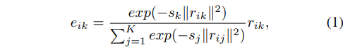
这里的softmax计算出了r前面的这个系数，得到的形状为NxHWxK。

# aggregate
E = aggregate(A, X, self.codewords)
class _aggregate(Function):
    @staticmethod
    def forward(ctx, A, X, C):
        # A \in(BxNxK) R \in(BxNxKxD) => E \in(BxNxD)
        ctx.save_for_backward(A, X, C)
        if A.is_cuda:
            E = lib.gpu.aggregate_forward(A, X, C)
        else:
            E = lib.cpu.aggregate_forward(A, X, C)
        return E
    @staticmethod
    def backward(ctx, gradE):
        A, X, C = ctx.saved_variables
        if A.is_cuda:
            gradA, gradX, gradC = lib.gpu.aggregate_backward(gradE, A, X, C)
        else:
            gradA, gradX, gradC = lib.cpu.aggregate_backward(gradE, A, X, C)
        return gradA, gradX, gradC
def aggregate(A, X, C):
    r""" Aggregate operation, aggregate the residuals of inputs (:math:`X`) with repect
    to the codewords (:math:`C`) with assignment weights (:math:`A`).
    .. math::
        e_{k} = \sum_{i=1}^{N} a_{ik} (x_i - d_k)
    Shape:
        - Input: 
          :math:`A\in\mathcal{R}^{B\times N\times K}`
          :math:`X\in\mathcal{R}^{B\times N\times D}` 
          :math:`C\in\mathcal{R}^{K\times D}`
          (where 
            :math:`B` is batch, 
            :math:`N` is total number of features,
            :math:`K` is number is codewords, 
            :math:`D` is feature dimensions.)
        - Output: 
          :math:`E\in\mathcal{R}^{B\times K\times D}`
    Examples:
        >>> B,N,K,D = 2,3,4,5
        >>> A = Variable(torch.cuda.DoubleTensor(B,N,K).uniform_(-0.5,0.5), requires_grad=True)
        >>> X = Variable(torch.cuda.DoubleTensor(B,N,D).uniform_(-0.5,0.5), requires_grad=True)
        >>> C = Variable(torch.cuda.DoubleTensor(K,D).uniform_(-0.5,0.5), requires_grad=True)
        >>> func = encoding.aggregate()
        >>> E = func(A, X, C)
    """
    return _aggregate.apply(A, X, C)

这里对权重进行聚合，得到每个样本对应的码本权重（？）。最终得到的大小为NxKxC。

Semantic Encoding Loss

标准的语义分割训练过程，使用的是逐像素的交叉熵，这将像素独立开学习。这样网络在没有全局上下文情况下可能会难以理解上下文，为了规范上下文编码模块的训练过程，使用Semantic Encoding Loss (SE-loss)在少量额外计算消耗的情况下强制网络理解全局语义信息。

在编码层之上添加了一个带Sigmoid激活的FC层用于单独预测场景中出现的目标类别，并学习二进制交叉熵损失。

不同于逐像素损失，SE-loss 对于大小不同的目标有相同的贡献，这能够提升小目标的检测性能。

class EncModule(nn.Module):
    def __init__(self, in_channels, nclass, ncodes=32, se_loss=True, norm_layer=None):
        super(EncModule, self).__init__()
...
        if self.se_loss:
            self.selayer = nn.Linear(in_channels, nclass)
    def forward(self, x):
...
        outputs = [F.relu_(x + x * y)]
        if self.se_loss:
            outputs.append(self.selayer(en))
        return tuple(outputs)
 class EncHead(nn.Module):
    def __init__(self, in_channels, out_channels, se_loss=True, lateral=True,
                 norm_layer=None, up_kwargs=None):
        super(EncHead, self).__init__()
...
        self.encmodule = EncModule(512, out_channels, ncodes=32,
            se_loss=se_loss, norm_layer=norm_layer)
        self.conv6 = nn.Sequential(nn.Dropout2d(0.1, False),
                                   nn.Conv2d(512, out_channels, 1))
    def forward(self, *inputs):
...
        outs = list(self.encmodule(feat))
        outs[0] = self.conv6(outs[0])
        return tuple(outs)

可以看出，在代码实现中使用的是相乘加权后的特征图进过一个FC之后进行的输出，而主干部分则是单独又进过 conv6 的处理进行了输出。与原始的结构图略有差异。

Context Encoding Network

在提出的上下文编码模块基础上，基于使用了扩张策略的预训练ResNet构建了Context Encoding Network (EncNet)。 扩张策略细节如下：

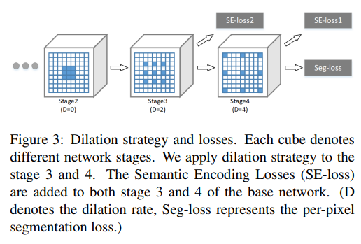
扩张策略：在stage3扩张2，stage4扩张4。

为了进一步的提升和规范上下文编码模块的训练，使用了单独的分离分支用于最小化SE-loss，该Loss采用已编码的语义作为输入并预测对象类别的存在。因为上下文模块和SE-loss是轻量级的，论文在stage3上端添加另一个上下文编码模块用于最小化SE-loss作为额外的正则化，这类比于PSPNet的辅助分支但比那个轻量了许多。SE-loss的ground truth是从真实的ground-truth分割mask上直接生成的。上下文编码模块插入到现存的CNN模型上是不需要额外的修正和监督的。
**
以下是官方代码的一个简单的EncNet。

class EncNet(BaseNet):
    def __init__(self, nclass, backbone, aux=True, se_loss=True, lateral=False,
                 norm_layer=SyncBatchNorm, **kwargs):
        super(EncNet, self).__init__(nclass, backbone, aux, se_loss,
                                     norm_layer=norm_layer, **kwargs)
        self.head = EncHead(2048, self.nclass, se_loss=se_loss,
                            lateral=lateral, norm_layer=norm_layer,
                            up_kwargs=self._up_kwargs)
        if aux:
            self.auxlayer = FCNHead(1024, nclass, norm_layer=norm_layer)
    def forward(self, x):
        imsize = x.size()[2:]
        features = self.base_forward(x)
        x = list(self.head(*features))
        x[0] = F.interpolate(x[0], imsize, **self._up_kwargs)
        if self.aux:
            auxout = self.auxlayer(features[2])
            auxout = F.interpolate(auxout, imsize, **self._up_kwargs)
            x.append(auxout)
        return tuple(x)

可以看出主要的EncNet的结构：self.base_forward -> self.head -> interpolate -> output

class EncModule(nn.Module):
    def __init__(self, in_channels, nclass, ncodes=32, se_loss=True, norm_layer=None):
        super(EncModule, self).__init__()
        self.se_loss = se_loss
        self.encoding = nn.Sequential(
            nn.Conv2d(in_channels, in_channels, 1, bias=False),
            norm_layer(in_channels),
            nn.ReLU(inplace=True),
            Encoding(D=in_channels, K=ncodes),  # 输出 NxKxC
            norm_layer(ncodes),
            nn.ReLU(inplace=True),
            Mean(dim=1))  # 在维度1上计算均值，得到最终的e NxC
        self.fc = nn.Sequential(
            nn.Linear(in_channels, in_channels),
            nn.Sigmoid())
        if self.se_loss:
            self.selayer = nn.Linear(in_channels, nclass)
    def forward(self, x):
        en = self.encoding(x)
        b, c, _, _ = x.size()
        gamma = self.fc(en)  # 得到要加权在CNN特征上的权重向量
        y = gamma.view(b, c, 1, 1)
        outputs = [F.relu_(x + x * y)]  # 如此加权，如何理解？
        if self.se_loss:
            outputs.append(self.selayer(en))  # 可计算se-loss
        return tuple(outputs)
class EncHead(nn.Module):
    def __init__(self, in_channels, out_channels, se_loss=True, lateral=True,
                 norm_layer=None, up_kwargs=None):
        super(EncHead, self).__init__()
        self.se_loss = se_loss
        self.lateral = lateral
        self.up_kwargs = up_kwargs
        self.conv5 = nn.Sequential(
            nn.Conv2d(in_channels, 512, 3, padding=1, bias=False),
            norm_layer(512),
            nn.ReLU(inplace=True))
        if lateral:
            self.connect = nn.ModuleList([
                nn.Sequential(
                    nn.Conv2d(512, 512, kernel_size=1, bias=False),
                    norm_layer(512),
                    nn.ReLU(inplace=True)),
                nn.Sequential(
                    nn.Conv2d(1024, 512, kernel_size=1, bias=False),
                    norm_layer(512),
                    nn.ReLU(inplace=True)),
            ])
            self.fusion = nn.Sequential(
                    nn.Conv2d(3*512, 512, kernel_size=3, padding=1, bias=False),
                    norm_layer(512),
                    nn.ReLU(inplace=True))
        self.encmodule = EncModule(512, out_channels, ncodes=32,
            se_loss=se_loss, norm_layer=norm_layer)
        self.conv6 = nn.Sequential(nn.Dropout2d(0.1, False),
                                   nn.Conv2d(512, out_channels, 1))
    def forward(self, *inputs):
        feat = self.conv5(inputs[-1])
        # 添加了两条额外的支路，都是1x1卷积进行调整后的结果
        if self.lateral:
            c2 = self.connect[0](inputs[1])
            c3 = self.connect[1](inputs[2])
            feat = self.fusion(torch.cat([feat, c2, c3], 1))
        outs = list(self.encmodule(feat))
        outs[0] = self.conv6(outs[0])
        return tuple(outs)

可以看出来，对于EncHead就是一个接在基础网络后的添加编码部分的一个区块。其中通过 outs = list(self.encmodule(feat)) 来添加了编码层。编码之后进行了一个2d的dropout和卷积，来进一步融合特征。

Featuremap Attention

为了使用编码层捕获的编码语义，预测一组特征图的放缩因子用于突出需要强调的类别。在编码层端上使用FC层，使用sigmoid作为激活函数，预测特征图的放缩因子γ=δ(We)，其中W表示层的权重，δ表示sigmoid激活函数。模块通过Y=X⊗γ得到输出，每个通道在特征图X和放缩因子γ之间做逐像素相乘。

en = self.encoding(x)
b, c, _, _ = x.size()
gamma = self.fc(en)  # 得到要加权在CNN特征上的权重向量
y = gamma.view(b, c, 1, 1)
outputs = [F.relu_(x + x * y)]  # 如此加权，如何理解？

这样的方法受SE-Net等工作的启发，即考虑强调天空出现飞机，不强调出现车辆的可能性。

Relation to Other Approaches

Segmentation Approaches

CNN在包括语义分割的计算机视觉领域上成为了标准方法。FCN开创了端到端的训练方式，但是因为在图像分类任务上预训练导致的特征图空间分辨率的损失，语义分割任务需要恢复细节信息。

1. 有工作是学习上采样滤波器，即decoder等
2. 另一个方法是使用扩张卷积保持较大的感受野生成密集预测

早期有使用CRF做后端处理，也实现了端对端训练；最近基于FCN架构通过大扩张率卷积或全局/金字塔池化提升接受野达到性能上的提升。

Prior work adopts dense CRF taking FCN outputs to refine the segmentation boundaries, and CRF-RNN achieves end-to-end learning of CRF with FCN. Recent FCN-based work dramatically boosts performance by increasing the receptive field with larger rate atrous convolution or global/pyramid pooling.

这些策略是以牺牲模型效率为代价：

1. 例如PSPNet在PSP模块和上采样后对平面特征图使用卷积
2. DeepLab使用大扩张率卷积在极端情况下会退化为1×1卷积

我们提出的上下文编码模块能够有效的利用全局上下文用作语义分割。这只需要少量的计算消耗成本。

Featuremap Attention and Scaling

逐通道式的特征attention是受到其他工作启发。

1. Spatial Transformer Network在没有额外监督的条件下在网络内部学习了空间变换。
2. Batch Normalization 是的小批量数据的均值和方差作为网络的一部分做标准化，成功的允许使用更大的学习率，并使得网络对初始方法不是那么敏感。
3. 最近在风格转换方面的工作处理特征图均值和方差或二阶统计信息用于启动网络内部风格变换。
4. 最近的SE-Net探究了跨通道信息以学习逐通道attention。

受这些方法启发，论文使用以编码语义预测特征图通道的放缩因子，这提供了在给定场景上下文的情况下强调个别特征图的机制。

实验细节

基础层使用带扩张卷积策略的预训练ResNet，最终输出为输入的1/8。使用双线性上采样到指定大小并计算loss。

实际情况下，越大的crop尺度对语义分割任务性能更好，但这同时需要更大的GPU存储空间，相应的这会减少Batch Normalization的batchsize，弱化训练过程。

为了解决这个问题，论文在PyTorch中实现了跨GPU的Sync-BN，实际的训练过程中使用batchsize为16。

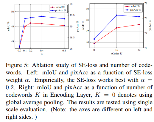
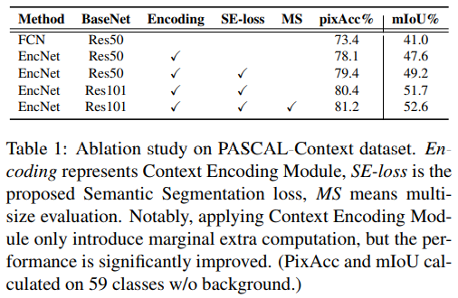
论文以Dilated ResNet FCN为对比的baseline。对于训练的EncNet，在编码层使用32个codewords，SE-loss的ground truth通过在给定的ground-truth 分割mask中通过”unique”操作查找类别，最终的loss是逐像素loss和SE-Loss的加权和。

使用了Poly方式的衰减。

参考链接

• https://blog.csdn.net/u011974639/article/details/79806893
• http://openaccess.thecvf.com/content_cvpr_2018/papers/Zhang_Context_Encoding_for_CVPR_2018_paper.pdf
• https://github.com/zhanghang1989/PyTorch-Encoding