这里将会总结关于S2-MLP的两篇文章。这两篇文章核心思路是一样的,即基于空间偏移操作替换空间MLP。
从摘要理解文章
V1
Recently, visual Transformer (ViT) and its following works abandon the convolution and exploit the self-attention operation, attaining a comparable or even higher accuracy than CNNs. More recently, MLP-Mixer abandons both the convolution and the self-attention operation, proposing an architecture containing only MLP layers.
To achieve cross-patch communications, it devises an additional token-mixing MLP besides the channel-mixing MLP. It achieves promising results when training on an extremely large-scale dataset. But it cannot achieve as outstanding performance as its CNN and ViT counterparts when training on medium-scale datasets such as ImageNet1K and ImageNet21K. The performance drop of MLP-Mixer motivates us to rethink the token-mixing MLP.
这里引出了本文的主要内容,即改进空间MLP。
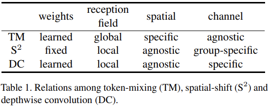
We discover that the token-mixing MLP is a variant of the depthwise convolution with a global reception field and spatial-specific configuration. But the global reception field and the spatial-specific property make token-mixing MLP prone to over-fitting.
指出了空间MLP的问题,由于其全局感受野和空间特定的属性使得模型容易过拟合。
In this paper, we propose a novel pure MLP architecture, spatial-shift MLP (S2-MLP). Different from MLP-Mixer, our S2-MLP only contains channel-mixing MLP.
这里提到仅有通道MLP,说明想到了新的办法来扩张通道MLP的感受野还可以保留点运算。
We utilize a spatial-shift operation for communications between patches. It has a local reception field and is spatial-agnostic. It is parameter-free and efficient for computation.
引出本文的核心内容,也就是标题中提到的空间偏移操作。看上去这一操作不带参数,仅仅是用来调整特征的一个处理手段。 Spatial-Shift操作可以参考这里的几篇文章:https://www.yuque.com/lart/architecture/conv#i8nnp
NewConv
The proposed S2-MLP attains higher recognition accuracy than MLP-Mixer when training on ImageNet-1K dataset. Meanwhile, S2-MLP accomplishes as excellent performance as ViT on ImageNet-1K dataset with considerably simpler architecture and fewer FLOPs and parameters.
V2
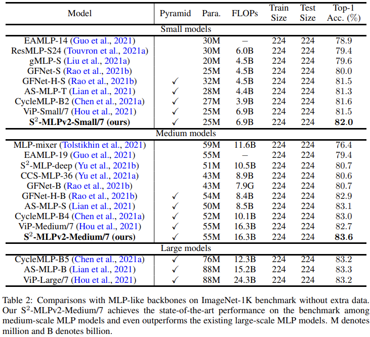
Recently, MLP-based vision backbones emerge. MLP-based vision architectures with less inductive bias achieve competitive performance in image recognition compared with CNNs and vision Transformers. Among them, spatial-shift MLP (S2-MLP), adopting the straightforward spatial-shift operation, achieves better performance than the pioneering works including MLP-mixer and ResMLP. More recently, using smaller patches with a pyramid structure, Vision Permutator (ViP) and Global Filter Network (GFNet) achieve better performance than S2-MLP.
这里引出了金字塔结构,看来V2版本要使用类似的构造。
In this paper, we improve the S2-MLP vision backbone. We expand the feature map along the channel dimension and split the expanded feature map into several parts. We conduct different spatial-shift operations on split parts.
依然延续了空间偏移的策略,但是不知道相较于V1版本改动如何
Meanwhile, we exploit the split-attention operation to fuse these split parts.
这里还引入了split-attention(ResNeSt)来融合分组。难道这里是要使用并行分支?
Moreover, like the counterparts, we adopt smaller-scale patches and use a pyramid structure for boosting the image recognition accuracy.
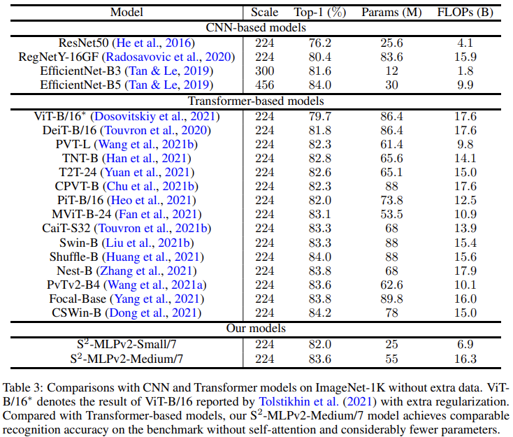
We term the improved spatial-shift MLP vision backbone as S2-MLPv2. Using 55M parameters, our medium-scale model, S2-MLPv2-Medium achieves an 83.6% top-1 accuracy on the ImageNet-1K benchmark using 224×224 images without self-attention and external training data.
在我看来,V2相较于V1,主要是借鉴了CycleFC的一些想法,并进行了适应性的调整。整体改动有两方面:
- 引入多分支处理的思想,并应用Split-Attention来融合不同分支。
- 受现有工作的启发,使用更小的patch和分层金字塔结构。
主要内容
核心结构比较
V1中,整体流程延续的是MLP-Mixer的思路,仍然保持直筒状结构。
MLP-Mixer的结构图:
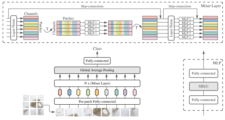
从图中可以看到,不同于MLP-Mixer中的Pre-Norm结构,S2MLP使用的是Post-Norm结构。
另外,S2MLP的改动主要集中在空间MLP的位置,由原来的Spatial-MLP(Linear->GeLU->Linear)转变为Spatial-Shifted Channel-MLP(Linear->GeLU->Spatial-Shift->Lienar)。
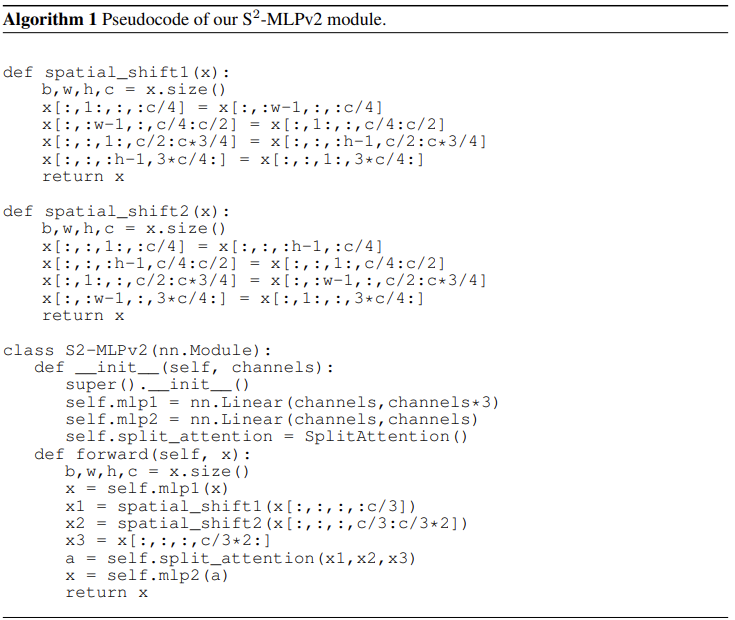
关于空间偏移的核心伪代码如下: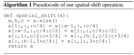
可以看到,这里就是将输入划分成四个不同的分组,各自沿着不同的轴向(H和W轴)偏移,由于实现的原因,在边界部分会有重复值出现。分组数依赖于方向的数量,这里默认使用4,即向四个方向偏移。
虽然从单个空间偏移模块上来看,仅仅关联了相邻的patch,但是从整体堆叠后的结构来看,可以实现一个近似的长距离交互过程。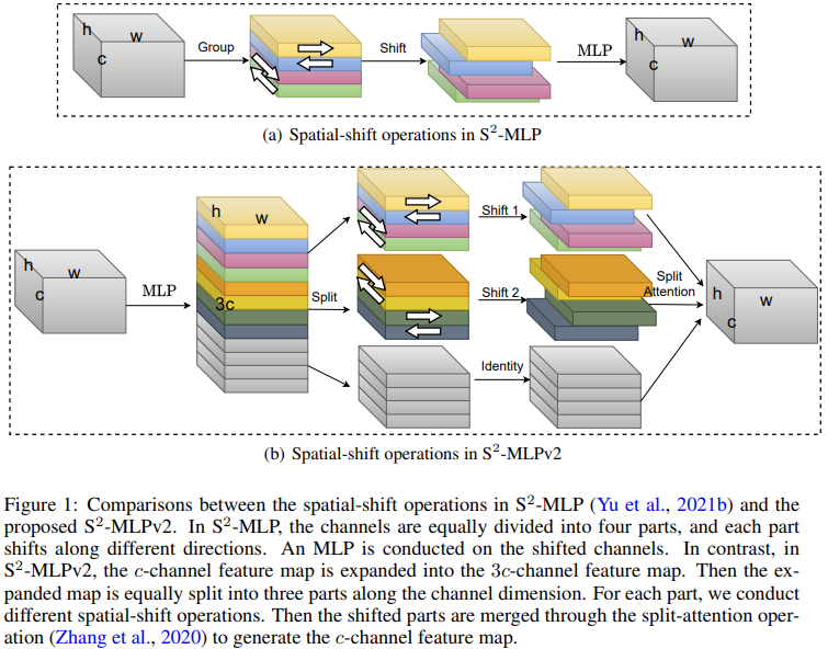
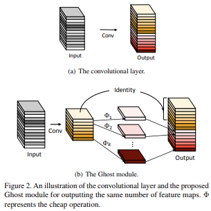
而在V2版本相较于V1版本引入了多分支处理的策略,并且在结构上开始使用Pre-Norm形式。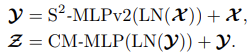
关于多分支结构的构造思路与CycleFC非常类似。不同支路使用不同的处理策略,同时在多分支整合时,使用了Split-Attention的方式进行融合。
Split-Attention: Vision Permutator (Hou et al., 2021) adopts split attention proposed in ResNeSt (Zhang et al., 2020) for enhancing multiple feature maps from different operations. 本文借鉴使用来融合多分支。 主要操作过程:
- 输入
个特征图(可以来自不同分支)
- 将所有特诊图的列求和后的结果累加:
- 通过堆叠的全连接层进行变换,得到针对不同特征图的通道注意力logits:
- 使用reshape来调整注意力向量的形状:
- 使用softmax沿着索引
计算,来获得针对不同样本的归一化注意力权重:
- 对输入的
个特征图加权求和得到结果
,其一行的结果可以表示为:


不过需要注意的是,这里第三个分支是一个恒等分支,直接将输入的部分通道取了过来,这一点延续了GhostNet的想法,而不同于CycleFC,使用的是一个独立的通道MLP。
GhostNet的核心结构:
其他细节
Spatial-Shift与Depthwise Convolution的关系
实际上,四个方向的偏移都是可以通过特定的卷积核构造来实现的: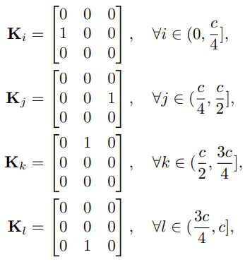
所以分组空间偏移操作可以通过为Depthwise Convolution的不同分组指定对应上面的卷积核来实现。
实际上实现偏移的方法非常多,除了文中提到的切片索引和构造核的depthwise convolution的方式,还可以通过分组torch.roll和自定义offset的deform_conv2d来实现。
import torchimport torch.nn.functional as Ffrom torchvision.ops import deform_conv2dxs = torch.meshgrid(torch.arange(5), torch.arange(5))x = torch.stack(xs, dim=0)x = x.unsqueeze(0).repeat(1, 4, 1, 1).float()direct_shift = torch.clone(x)direct_shift[:, 0:2, :, 1:] = torch.clone(direct_shift[:, 0:2, :, :4])direct_shift[:, 2:4, :, :4] = torch.clone(direct_shift[:, 2:4, :, 1:])direct_shift[:, 4:6, 1:, :] = torch.clone(direct_shift[:, 4:6, :4, :])direct_shift[:, 6:8, :4, :] = torch.clone(direct_shift[:, 6:8, 1:, :])print(direct_shift)pad_x = F.pad(x, pad=[1, 1, 1, 1], mode="replicate") # 这里需要借助padding来保留边界的数据roll_shift = torch.cat([torch.roll(pad_x[:, c * 2 : (c + 1) * 2, ...], shifts=(shift_h, shift_w), dims=(2, 3))for c, (shift_h, shift_w) in enumerate([(0, 1), (0, -1), (1, 0), (-1, 0)])],dim=1,)roll_shift = roll_shift[..., 1:6, 1:6]print(roll_shift)k1 = torch.FloatTensor([[0, 0, 0], [1, 0, 0], [0, 0, 0]]).reshape(1, 1, 3, 3)k2 = torch.FloatTensor([[0, 0, 0], [0, 0, 1], [0, 0, 0]]).reshape(1, 1, 3, 3)k3 = torch.FloatTensor([[0, 1, 0], [0, 0, 0], [0, 0, 0]]).reshape(1, 1, 3, 3)k4 = torch.FloatTensor([[0, 0, 0], [0, 0, 0], [0, 1, 0]]).reshape(1, 1, 3, 3)weight = torch.cat([k1, k1, k2, k2, k3, k3, k4, k4], dim=0) # 每个输出通道对应一个输入通道conv_shift = F.conv2d(pad_x, weight=weight, groups=8)print(conv_shift)offset = torch.empty(1, 2 * 8 * 1 * 1, 1, 1)for c, (rel_offset_h, rel_offset_w) in enumerate([(0, -1), (0, -1), (0, 1), (0, 1), (-1, 0), (-1, 0), (1, 0), (1, 0)]):offset[0, c * 2 + 0, 0, 0] = rel_offset_hoffset[0, c * 2 + 1, 0, 0] = rel_offset_woffset = offset.repeat(1, 1, 7, 7).float()weight = torch.eye(8).reshape(8, 8, 1, 1).float()deconv_shift = deform_conv2d(pad_x, offset=offset, weight=weight)deconv_shift = deconv_shift[..., 1:6, 1:6]print(deconv_shift)"""tensor([[[[0., 0., 0., 0., 0.],[1., 1., 1., 1., 1.],[2., 2., 2., 2., 2.],[3., 3., 3., 3., 3.],[4., 4., 4., 4., 4.]],[[0., 0., 1., 2., 3.],[0., 0., 1., 2., 3.],[0., 0., 1., 2., 3.],[0., 0., 1., 2., 3.],[0., 0., 1., 2., 3.]],[[0., 0., 0., 0., 0.],[1., 1., 1., 1., 1.],[2., 2., 2., 2., 2.],[3., 3., 3., 3., 3.],[4., 4., 4., 4., 4.]],[[1., 2., 3., 4., 4.],[1., 2., 3., 4., 4.],[1., 2., 3., 4., 4.],[1., 2., 3., 4., 4.],[1., 2., 3., 4., 4.]],[[0., 0., 0., 0., 0.],[0., 0., 0., 0., 0.],[1., 1., 1., 1., 1.],[2., 2., 2., 2., 2.],[3., 3., 3., 3., 3.]],[[0., 1., 2., 3., 4.],[0., 1., 2., 3., 4.],[0., 1., 2., 3., 4.],[0., 1., 2., 3., 4.],[0., 1., 2., 3., 4.]],[[1., 1., 1., 1., 1.],[2., 2., 2., 2., 2.],[3., 3., 3., 3., 3.],[4., 4., 4., 4., 4.],[4., 4., 4., 4., 4.]],[[0., 1., 2., 3., 4.],[0., 1., 2., 3., 4.],[0., 1., 2., 3., 4.],[0., 1., 2., 3., 4.],[0., 1., 2., 3., 4.]]]])tensor([[[[0., 0., 0., 0., 0.],[1., 1., 1., 1., 1.],[2., 2., 2., 2., 2.],[3., 3., 3., 3., 3.],[4., 4., 4., 4., 4.]],[[0., 0., 1., 2., 3.],[0., 0., 1., 2., 3.],[0., 0., 1., 2., 3.],[0., 0., 1., 2., 3.],[0., 0., 1., 2., 3.]],[[0., 0., 0., 0., 0.],[1., 1., 1., 1., 1.],[2., 2., 2., 2., 2.],[3., 3., 3., 3., 3.],[4., 4., 4., 4., 4.]],[[1., 2., 3., 4., 4.],[1., 2., 3., 4., 4.],[1., 2., 3., 4., 4.],[1., 2., 3., 4., 4.],[1., 2., 3., 4., 4.]],[[0., 0., 0., 0., 0.],[0., 0., 0., 0., 0.],[1., 1., 1., 1., 1.],[2., 2., 2., 2., 2.],[3., 3., 3., 3., 3.]],[[0., 1., 2., 3., 4.],[0., 1., 2., 3., 4.],[0., 1., 2., 3., 4.],[0., 1., 2., 3., 4.],[0., 1., 2., 3., 4.]],[[1., 1., 1., 1., 1.],[2., 2., 2., 2., 2.],[3., 3., 3., 3., 3.],[4., 4., 4., 4., 4.],[4., 4., 4., 4., 4.]],[[0., 1., 2., 3., 4.],[0., 1., 2., 3., 4.],[0., 1., 2., 3., 4.],[0., 1., 2., 3., 4.],[0., 1., 2., 3., 4.]]]])tensor([[[[0., 0., 0., 0., 0.],[1., 1., 1., 1., 1.],[2., 2., 2., 2., 2.],[3., 3., 3., 3., 3.],[4., 4., 4., 4., 4.]],[[0., 0., 1., 2., 3.],[0., 0., 1., 2., 3.],[0., 0., 1., 2., 3.],[0., 0., 1., 2., 3.],[0., 0., 1., 2., 3.]],[[0., 0., 0., 0., 0.],[1., 1., 1., 1., 1.],[2., 2., 2., 2., 2.],[3., 3., 3., 3., 3.],[4., 4., 4., 4., 4.]],[[1., 2., 3., 4., 4.],[1., 2., 3., 4., 4.],[1., 2., 3., 4., 4.],[1., 2., 3., 4., 4.],[1., 2., 3., 4., 4.]],[[0., 0., 0., 0., 0.],[0., 0., 0., 0., 0.],[1., 1., 1., 1., 1.],[2., 2., 2., 2., 2.],[3., 3., 3., 3., 3.]],[[0., 1., 2., 3., 4.],[0., 1., 2., 3., 4.],[0., 1., 2., 3., 4.],[0., 1., 2., 3., 4.],[0., 1., 2., 3., 4.]],[[1., 1., 1., 1., 1.],[2., 2., 2., 2., 2.],[3., 3., 3., 3., 3.],[4., 4., 4., 4., 4.],[4., 4., 4., 4., 4.]],[[0., 1., 2., 3., 4.],[0., 1., 2., 3., 4.],[0., 1., 2., 3., 4.],[0., 1., 2., 3., 4.],[0., 1., 2., 3., 4.]]]])tensor([[[[0., 0., 0., 0., 0.],[1., 1., 1., 1., 1.],[2., 2., 2., 2., 2.],[3., 3., 3., 3., 3.],[4., 4., 4., 4., 4.]],[[0., 0., 1., 2., 3.],[0., 0., 1., 2., 3.],[0., 0., 1., 2., 3.],[0., 0., 1., 2., 3.],[0., 0., 1., 2., 3.]],[[0., 0., 0., 0., 0.],[1., 1., 1., 1., 1.],[2., 2., 2., 2., 2.],[3., 3., 3., 3., 3.],[4., 4., 4., 4., 4.]],[[1., 2., 3., 4., 4.],[1., 2., 3., 4., 4.],[1., 2., 3., 4., 4.],[1., 2., 3., 4., 4.],[1., 2., 3., 4., 4.]],[[0., 0., 0., 0., 0.],[0., 0., 0., 0., 0.],[1., 1., 1., 1., 1.],[2., 2., 2., 2., 2.],[3., 3., 3., 3., 3.]],[[0., 1., 2., 3., 4.],[0., 1., 2., 3., 4.],[0., 1., 2., 3., 4.],[0., 1., 2., 3., 4.],[0., 1., 2., 3., 4.]],[[1., 1., 1., 1., 1.],[2., 2., 2., 2., 2.],[3., 3., 3., 3., 3.],[4., 4., 4., 4., 4.],[4., 4., 4., 4., 4.]],[[0., 1., 2., 3., 4.],[0., 1., 2., 3., 4.],[0., 1., 2., 3., 4.],[0., 1., 2., 3., 4.],[0., 1., 2., 3., 4.]]]])"""
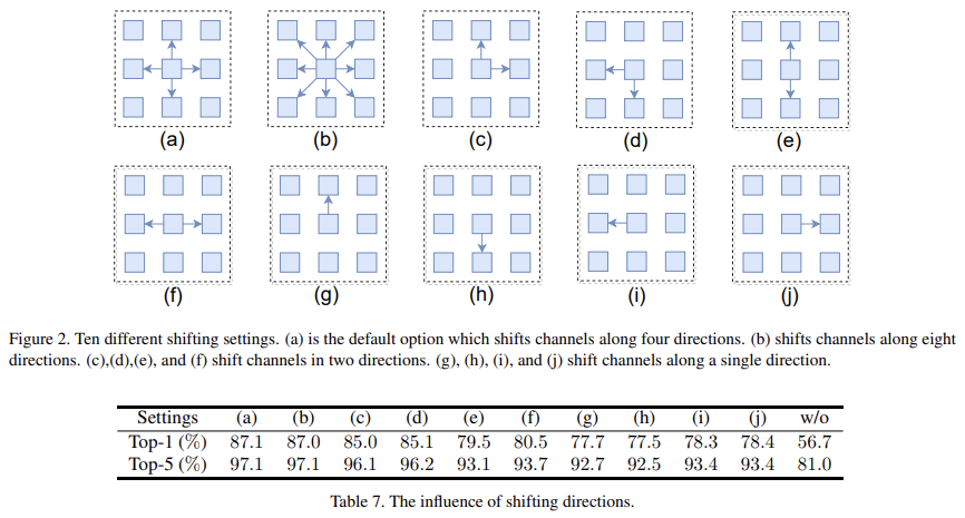
偏移方向的影响
实验是在ImageNet的子集上跑的。
V1中针对不同的偏移方向进行了消融实验,这里的模型中都是按照方向个数对通道分组。从结果中可以看到:
- 偏移确实可以带来性能增益。
- a和b:四个方向和八个方向相比,差异并不大。
- e和f:水平偏移效果更好。
-
输入尺寸以及patchsize的影响
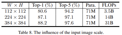
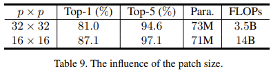
实验是在ImageNet的子集上跑的。
V1中在固定patchsize后,不同的输入尺寸WxH的表现也不同。过大的patchsize效果也不好,会丢失更多的细节信息,但是却可以有效提升推理速度。金字塔结构的有效性
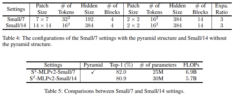
V2中,构造了两个不同的结构,一个有着更小的patch,并且使用金字塔结构,另一个更大的patch,不使用金字塔结构。可以看到,同时受益于小patchsize带来的细节信息的性能增强和金字塔结构带来的更优的计算效率,前者获得了更好的表现。Split-Attention的效果
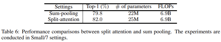
V2将split-attention与特征直接相加取平均对比。可以看到,前者更优。不过这里参数量也不一样了,其实更合理的比较应该最起码是加几层带参数的结构来融合三分支的特征。三分支结构的有效性
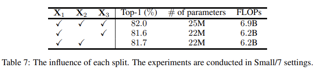
这里的实验说明有些模糊,作者说道“In this section, we evaluate the influence of removing one of them.”但是却没有说明去掉特定分支后其他结构的调整方式。实验结果
链接
论文:
- 参考代码:
- CycleFC的代码有可以借鉴之处: https://github.com/ShoufaChen/CycleMLP/blob/main/cycle_mlp.py

若有收获,就点个赞吧
0 人点赞
