背景知识

Guo Weilong教授于2013年发表了BSseeker2，又在2018年发表了CGmaptools，怎么来说呢，两个软件的联系是很紧密的，当时作者的想法也是想着这两个软件包揽DNA甲基化测序数据的上下游分析吧，不过软件确实是好软件，好多实用功能，建议系统学习一遍。

CGmaptools主页：https://cgmaptools.github.io/；
这是备份的说明文档地址：https://cgmaptools.github.io/zh/CGmapTools_zh.html

这是他们课题组为BS-seeker2 和 CGmapTools 写的一份简要使用说明：
重亚硫酸盐测序数据基本分析流程代码及软件：BS-seeker2 & CGmapTools
截图：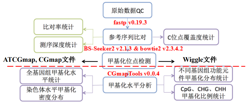

Tips：
cgmaptools的开发语言是python，而且是基于python2进行开发的，目前还没有更新到python3的cgmaptools，所以cgmaptools的绝大部分模块可能都需要在python2的环境下运行，建议使用conda新建一个python2的环境来管理cgmaptools。

逐个功能讲解

注：这里目前只有cgmaptools几个功能的笔记，有待填补。
不过总的来说，看软件说明书是最好的，因为软件作者可能随时更新而且还能随时提问，而大部分博客的笔记可能就更新没那么及时了。

4 SNV calling

亚硫酸氢盐测序数据包含甲基化和基因组序列的信息。除了 DNA 甲基化分析之外，我们还可以使用亚硫酸氢盐数据调用变体。由于在文库制备过程中亚硫酸氢盐覆盖和 PCR 扩增，DNA 片段上未甲基化的胞嘧啶将转化为胸腺嘧啶。因此，很难将亚硫酸氢盐覆盖产生的胸腺嘧啶与真正的胸腺嘧啶等位基因区分开来。
近年来，很少有工具适用于 SNP 调用的亚硫酸氢盐数据。主要思想是删除可能在给定位置含有未甲基化胞嘧啶的模糊读数。因此，其余读数可被视为从未经亚硫酸氢盐处理的正常基因组 DNA 生成的读数，并可用于使用常规方法调用变体，而无需考虑亚硫酸氢盐转化。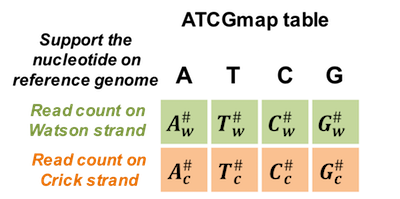

图 4.1：用于 SNV 调用的 ATCGmap 表
然而，在大多数情况下，去除模糊读段（vague reads）会导致信息丢失，从而降低变异调用的可信度，尤其是在测序深度较低的情况下。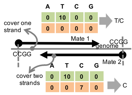

图 4.2：比对指代模糊基因型的示例
为了解决这个问题，我们尝试在基因型检测中引入通配符。即使对于这些模棱两可的基因型，我们仍然可以学到一些东西。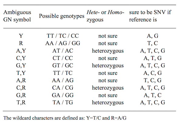

图 4.3：模糊基因型定义表
我们提出了两种独立的方法，称为 BinomWC（基于二项式）和 BayesWC（基于贝叶斯），同时考虑了模糊读段（vague reads）。

实战
使用cgmaptools snvcalling SNV。

cgmaptools snv -i T1N1.ATCGmap.gz -m bayes -v T1N1.bayes.vcf -o T1N1.bayes.snv --bayes-dynamicP
cgmaptools snv -i T1N1.ATCGmap.gz -m binom -o T1N1.binom.snv

获得了VCF格式的文件后，可以使用cgmaptools asm对突变进行可视化，实测耗时非常久。

RefGenome_rrbs=/mnt/MD3400/data003/lianzhiwei/01project/00RefandAnno/ref_genome_fa/Mus_musculus/ENSEMBL/GRCm38_release102/DNA/Mus_musculus.GRCm38.dna.primary_assembly.fa
# cgmaptools asm 命令的基础使用
cgmaptools asm -r ${RefGenome_rrbs} -b T1N1_merge4S.sorted.bam -l T1N1.bayes.vcf > T1N1.asm

snv格式

#chr    nuc     pos     ATCG_watson     ATCG_crick      predicted_nuc   p_value
1       G       3020796 16,0,0,7        2,0,0,1 A,G     3.0e-03
1       G       3020803 16,0,0,7        2,0,0,1 A,G     3.0e-03
1       G       3020804 16,0,0,7        2,0,0,1 A,G     3.0e-03
1       G       3020806 16,0,0,7        2,0,0,1 A,G     3.0e-03

vcf格式

##fileformat=VCFv4.2
##fileDate=20211110
##source=CGmapTools
##INFO=<ID=NS,Number=1,Type=Integer,Description="Number of Samples With Data">
##INFO=<ID=DP,Number=1,Type=Integer,Description="Total Depth">
##INFO=<ID=GU,Number=.,Type=String,Description="Genotype is Unidentified:R=A/G, Y=T/C">
##FILTER=<ID=q10,Description="Quality below 10">
##FORMAT=<ID=GT,Number=1,Type=String,Description="Genotype">
##FORMAT=<ID=GQ,Number=1,Type=Integer,Description="Genotype Quality">
##FORMAT=<ID=DP,Number=1,Type=Integer,Description="Read Depth">
#CHROM  POS     ID      REF     ALT     QUAL    FILTER  INFO    FORMAT  NA00001
1       3020796 .       G       A       0       PASS    NS=1:DP=26      GT:GQ:DP        0/1:0:26
1       3020803 .       G       A       0       PASS    NS=1:DP=26      GT:GQ:DP        0/1:0:26
1       3020804 .       G       A       0       PASS    NS=1:DP=26      GT:GQ:DP        0/1:0:26
1       3020806 .       G       A       0       PASS    NS=1:DP=26      GT:GQ:DP        0/1:0:26
1       3020807 .       G       A       0       PASS    NS=1:DP=42      GT:GQ:DP        0/1:0:42

5 Methylation Analysis

CGmapTools支持差异甲基化位点(DMS)分析和差异甲基化区域(DMR)分析。
由于现有的DNA甲基组要么是低覆盖率(如WGBS)，要么是在覆盖区域片段化(如RRBS)。在CGmapTools中，我们提出了一种新的方法动态片段策略来识别两个CGmap文件之间的dmr。

注意分析时的细节：
输入文件是由cgmaptools intersect命令获取，文件谁在前谁在后就决定了差异分析时的组别；所以建议文件名包含两个样本的信息。

番外：DSS包的DM（different methylation）检测策略
基于对 beta-二项式分布的严格 Wald 检验。其说明文档描述如下：
为了检测差异甲基化，在每个 CpG 位点进行统计测试，然后根据用户指定的阈值调用差异甲基化位点 (DML) 或差异甲基化区域 (DMR)。严格的统计测试应考虑重复和测序深度之间的生物学差异。大多数现有的 DM 分析方法都基于临时方法。例如，使用 Fisher 精确忽略生物变异，使用 t 检验估计甲基化水平忽略测序深度。有时会实现任意过滤：过滤掉深度低于任意阈值的轨迹，导致信息丢失
在 DSS 中实施的 DM 检测程序基于对 beta-二项式分布的严格 Wald 检验。测试统计取决于生物变异（以离散参数为特征）以及测序深度。该算法的一个重要部分是离散参数的估计，这是通过基于贝叶斯分层模型的收缩估计器实现的（Feng、Conneely 和 Wu 2014）。DSS 的一个优点是即使没有生物学重复也可以进行测试。这是因为通过平滑，相邻的 CpG 位点可以被视为伪复制，并且仍然可以以合理的精度估计离散度。
DSS 也适用于一般实验设计，基于具有反正弦链接函数的 beta-二项式回归模型。采用广义最小二乘法对变换后的数据进行模型拟合，与基于广义线性模型的方法相比，计算性能大大提高。

5.1 dms

差异甲基化位点分析，支持卡方和Fisher检验（Chi-square and Fisher tests）。

5.1.1 命令

#   Usage: cgmaptools dms [-i <CGmapInter>] [-m 5 -M 100] [-o output]
#         (aka CGmapInterDiffSite)
#   Description: 
#     Get the differentially methylated sites for two samples.
#   Input Format, same as the output of CGmapIntersect.py:
#       Chr1  C  3541  CG  CG  0.8  4  5  0.4  4  10
# 获取方式：cgmaptools intersect -h
#   Output Format:
#      chr1 C   4654    CG  CG  0.92    1.00    8.40e-01
#      chr1 C   4658    CHH CC  0.50    0.00    3.68e-04
#      chr1 G   8376    CG  CG  0.62    0.64    9.35e-01
#   
#   Options:
#     -h, --help            show this help message and exit
#     -i FILE               File name for CGmapInter, STDIN if omitted
#     -m INT, --min=INT     min coverage [default : 0]
#     -M INT, --max=INT     max coverage [default : 100]
#     -o OUTFILE            To standard output if omitted. Compressed output if
#                           end with .gz
#     -t STRING, --test-method=STRING
#                           chisq, fisher [default : chisq]

Example
cgmaptools dms -i intersect_CG.gz -m 4 -M 100 -o DMS.gz -t fisher

Output format
Example

chr1    C   4654    CG  CG  0.92    1.00    8.40e-01
chr1    C   4658    CHH CC  0.50    0.00    3.68e-04
chr1    G   8376    CG  CG  0.62    0.64    9.35e-01

Column Description

Figure 5.1: Output format description for cgmaptools dms

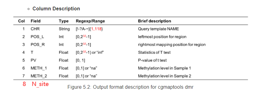
5.2 dmr

差异甲基化区域分析，使用动态片段策略。英文：Differentially methylated region analysis, using dynamic fragmentation strategy .
特点：

动态片段策略（Dynamic Fragment Strategy）
输出文件中有P value，可用于DMR的筛选和绘制火山图等；
只能两组中找差异，不支持多组/多因素的组别设置；

5.2.1 命令

#   Usage: cgmaptools dmr [-i <CGmapInter>] [-m 5 -M 100] [-o output]
#         (aka CGmapInterDiffReg)
#   Description: 
#     Get the differentially methylated regions using dynamic fragment strategy.
#   Input Format, same as the output of CGmapIntersect.py:
#      chr1  C  3541  CG  CG  0.8  4  5  0.4  4  10
#   Output Format, Ex:
#     #chr      start   end     t       pv          mC_A    mC_B    N_site
#      chr1    1004572 1004574 inf     0.00e+00    0.1100   0.0000  20
#      chr1    1009552 1009566 -0.2774 8.08e-01    0.0200   0.0300  15
#      chr1    1063405 1063498 0.1435  8.93e-01    0.6333   0.5733  5
#   Options:
#     -h, --help            show this help message and exit
#     -i FILE               File name for CGmapInter, STDIN if omitted
#     -c INT, --minCov=INT  min coverage [default : 4]    #单个CpGs的最低coverage
#     -C INT, --maxCov=INT  max coverage [default : 500]    #单个CpGs的最高coverage
#     -s INT, --minStep=INT
#                           min step in bp [default : 100]
#     -S INT, --maxStep=INT
#                           max step in bp [default : 1000]
#     -n INT, --minNSite=INT
#                           min N sites [default : 5]    #一个fragment内至少包含的CpGs数目
#     -o OUTFILE            To standard output if omitted. Compressed output if
#                           end with .gz
# 注：参数如有不理解的可以看看下面的“动态片段策略（Dynamic Fragment Strategy）说明图”

Example
cgmaptools dmr -i intersect_CG.gz -o DMR.gz

5.2.2 补充说明

输入格式

#Input Format, same as the output of CGmapIntersect.py:
chr1  C  3541  CG  CG  0.8  4  5  0.4  4  10

获取方式：cgmaptools intersect -h

输出格式

#chr      start   end     t       pv          mC_A    mC_B    N_site
chr1    1004572 1004574 inf     0.00e+00    0.1100   0.0000  20
chr1    1009552 1009566 -0.2774 8.08e-01    0.0200   0.0300  15
chr1    1063405 1063498 0.1435  8.93e-01    0.6333   0.5733  5

动态片段策略（Dynamic Fragment Strategy）

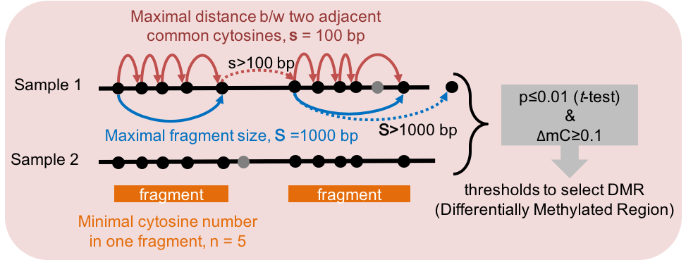
Figure 5.3: Dynamic Fragmentation Strategy

实战

两个样本的测试代码 ```bash cgmaptools intersect -1 T1N1_merge4S.mincov1.possort.CGmap -2 T1N2_merge4S.mincov1.possort.CGmap -o T1N1_vs_T1N2.intersect.CGmap

cgmaptools dmr -i T1N1_vs_T1N2.intersect.CGmap -o DMR_T1N1_vs_T1N2.txt.gz

使用shell统计有多少个显著差异的DMR
```bash
zcat DMR_T1N1_vs_T1N2.txt.gz | awk 'delta=$6-$7{if($5<0.01 && delta>0.1) print}' | wc -l
1327
zcat DMR_T1N1_vs_T1N2.txt.gz | awk 'delta=$6-$7{if($5<0.01 && delta<-0.1) print}' | wc -l
737
# Tips: 学习一下awk中定义函数，比如下面这条命令取数值的绝对值
zcat DMR_T1N1_vs_T1N2.txt.gz | awk -F'\t' 'function abs(v) {return v < 0 ? -v : v}{if(abs($6-$7)>0.1 && $5<=0.01) print}' | wc -l
2065

Tips
从CGmaptools GitHub上关于dmr功能的提问发现，有几个值得注意的地方，列举几个：

**cgmaptools dmr**的原始输出没有经过任何过滤，提供的是所有区域。

原始输出结果中，有的区域长度极短，因为cgmaptools dmr计算的策略是根据位点和步长来决定一个fragment是否应该输出的。以下是我做的一次测试的结果，可见有一个区域只有9bp长也被输出了。

#chr      start   end     t       pv          mC_A    mC_B    N_site    length
chr1    66017091        66017187        0.0456  9.65e-01        0.6920  0.6820  5       96
chr1    66175060        66175235        -1.2037 2.41e-01        0.0092  0.0200  12      175
chr1    66175434        66175645        -0.7545 4.55e-01        0.0100  0.0127  22      211
chr1    66468047        66468577        1.7407  8.33e-02        0.1246  0.0865  98      530
chr1    66521071        66521169        -0.1477 8.84e-01        0.9275  0.9325  12      98
chr1    66569856        66569892        -1.6624 1.27e-01        0.7167  0.9350  6       36
chr1    66659669        66659678        -0.1877 8.55e-01        0.9283  0.9350  6       9
chr1    66700832        66700850        -1.6348 1.28e-01        0.0014  0.0114  7       18
chr1    66701272        66701342        1.1523  2.64e-01        0.0050  0.0020  10      70

既然原始输出包含所有的位点根据一定原则输出的区域，那我们该如何选择有意义的dmr？
作者建议使用您认为合适的标准过滤它们。比如甲基化水平差异大于等于10%，并且p value < 0.01，这dmr输出结果中体现为|delta mC| >=0.1, p value < 0.01。
另外，CGmapTools和CGmap文件将区分CpG二核苷酸的链。因此，对于一个CpG二核苷酸，在不同的链上会有两个CG位点。
提问地址：Can you tell me how this become 6 CpG site? Seems logic error!!! #34

cgmaptools merge

如何使用两个以上的样本进行 DMS 或 DMR：例如 (样本1,样本2) vs. (样本3, 样本4)。

cgmaptools merge2 cgmap # for merging two CGmap files to one CGmap file
cgmaptools mergelist tosingle # for merging multiple CGmap files into one CGmap file.
另外，用户可以选择将cgmaptools dmr预测的dmr区域进行合并，意思是，如果两个dmr距离很近，那么就把它们合并为一个dmr。但是如何根据指定距离阈值来合并区域，我还没有想到解决办法。

提问地址：Annotating DMR/DMS #16

5.3 asm

使用精确预测的杂合子 SNVs (cgmaptools snv的运行结果)为输入，cgmaptools可以从BAM文件中识别等位基因特异性甲基化(ASM)区域。
输入文件之一是cgmaptools snv的运行结果，所以建议先去看看cgmaptools snv；

5.3.1 命令

#   DESCRIPTION
#           Allele specific methylated region/site calling
#           * Fisher exact test for site calling.
#           * Students' t-test for region calling.
#   
#   USAGE
#           cgmaptools asm [options] -r <ref.fa> -b <input.bam> -l <snp.vcf>
#           (aka ASM)
#   
#           Options:
#           -r    Samtools indexed reference genome seqeunce, fasta format. eg. hg19.fa
#                 - use samtools to index reference first: samtools faidx hg19.fa
#           -b    Samtools indexed Bam format file.
#                 - use samtools to index bam file first: samtools index <input.bam>
#           -l    SNPs in vcf file format.
#           -s    Path to samtools eg. /home/user/bin/samtools
#                 - by defualt, we try to search samtools in your system PATH,
#           -o    Output results to file. [default: STDOUT]
#           -t    C context. [default: CG]
#                 - available context: C, CG, CH, CW, CC, CA, CT, CHG, CHH
#           -m    Specify calling mode. [default: asr]
#                 - alternative: ass
#                 - asr: allele specific methylated region
#                 - ass: allele specific methylated site
#           -d    Minimum number of read for each allele linked site to call ass. [default: 3]
#                 - ass specific.
#           -n    Minimum number of C site each allele linked to call asr. [default: 2]
#                 - asr specific.
#           -D    Minimum read depth for C site to call methylation level when calling asr. [default: 1]
#                 - asr specific.
#           -L    Low methylation level threshold. [default: 0.2]
#                 - allele linked region [or site] with low methylation level should be no greater than this threshold.
#           -H    High methylation level threshold. [default: 0.8]
#                 - allele linked region[or site] with high methylation level should be no less than this threshold.
#           -q    Adjusted p value using Benjamini & Hochberg (1995) ("BH" or its alias "fdr"). [default: 0.05]
#           -h    Help message.

Example

gawk '{if(/^#/){print}else{print "chr"$0;}}' bayes.vcf > bayes2.vcf
cgmaptools asm -r genome.fa -b WG.bam -l bayes2.vcf > WG.asm

Output format 1: for ASS (Allele-Specific methylated Site)

Example

Chr    SNP_Pos  Ref    Allele1     Allele2      C_Pos   Allele1_linked_C    Allele2_linked_C    Allele1_linked_C_met    Allele2_linked_C_met    pvalue   fdr    ASM
Chr1    8949221 T         T             A           8949252 30,2    6,0 0.94    1.00          1.00e+00         1.00e+00      FALSE
Chr1    8965481 A         A            T               8965494  12,3    12,4    0.80    0.75          1.00e+00         1.00e+00      FALSE

Column Description

Figure 5.5: Output format description for cgmaptools asm -m ass

Output format 2: for ASR (Allele-Specific methylated Region)

Chr        Pos          Ref   Allele1   Allele2       Allele1_linked_C   Allele2_linked_C  Allele1_linked_C_met   Allele2_linked_C_met   pvalue      fdr             ASM
chr1       8943402   A        A        T                      1-1                         0.8-1                        1              0.9                        5.01e-01   7.52e-01    FALSE
chr1       8966879   C        C        G                    0.93-0-0     0.81-0-0         0.31            0.27                       9.27e-01    9.53e-01   FALSE

Column Description

Figure 5.6: Output format description for cgmaptools asm -m asr

5.4 mbed

cgmaptools mbed将为所有感兴趣区域（按照染色体为单位）计算出一个DNA甲基化水平，这与cgmaptools mtr不同。
例如，该功能可用于计算启动子、基因体、特定转座子元件(TEs)等区域的平均DNA甲基化水平。

5.1.1 命令

#   Usage:  cgmaptools mbed [-i <CGmap>]  -b <regin.bed> [-c 5 -C 500 -s] 
#         (aka CGmapMethylInBed)
#   Description: Calculated bulk average methylation levels in given regions.
#   Options:
#      -i  String, CGmap file; use STDIN if not specified
#          Please use "gunzip -c <input>.gz " and pipe as input for gzipped file.
#          Ex: chr1 G   3000851 CHH CC  0.1 1   10
#      -b  String, BED file, should have at least 4 columns
#          Ex: chr1 3000000 3005000 -
#      -c  Int, minimum Coverage [Default: 5] 
#      -C  Int, maximum Coverage [Default: 500] 
#      -s  Strands would be distinguished when specified
#      -h  help
#   
#   Output to STDOUT: #不知道为何作者写的是这个，输出格式其实是下面这种有七列的汇总表
#       Title         Count    mean_mC
#       sense         34       0.2353
#       antisense     54       0.2778
#       total         88       0.2614
#   Notice:
#       The overlapping of regions would not be checked. 
#       A site might be considered multiple times.

Example
cgmaptools mbed -i WG.CGmap -b region.bed >WG.mbed

Output format
示例，注意列的含义

#chr   sense_Count   sense_mC    anti_Count  anti_mC all_Count   all_mC
chr1    203   0.08127     178     0.1148      381     0.09692
chr2    185   0.07045     257     0.05586     442     0.06197
chr3    313   0.1042      250     0.1358      563     0.1182
chr4    300   0.1218      271     0.13      571   0.1257
chr5    282   0.1272      222     0.1589      504     0.1412

5.5 mbin

该函数将计算单个样本在等长的bins中的平均甲基化水平，并生成总结表和分布图。bins的取值范围来自于输入文件的基因组大小。
WGBS这种全基因组覆盖的测序数据比较合适绘制这种图，RRBS的话因为基因组覆盖区域很有限，所以很难绘制出满意的这种图。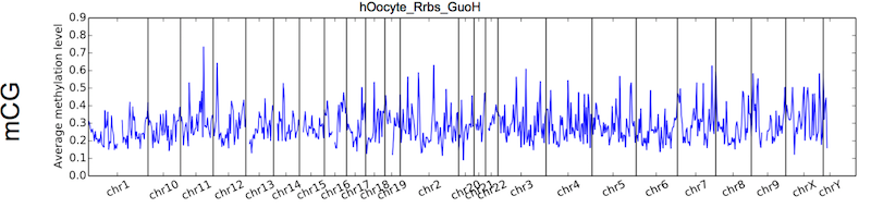

Figure 5.7: Output figure example for cgmaptools mbin
5.5.1 命令

#   Usage: cgmaptools mbin [-i <CGmap>] [-c 10 --CXY 5 -B 5000000] 
#         (aka CGmapMethInBins)
#   Description: Generate the methylation in Bins.
#   Output Ex:
#      chr1    1       5000    0.0000
#      chr1    5001    10000   0.0396
#      chr2    1       5000    0.0755
#      chr2    5001    10000   0.0027
#      chr3    1       5000    na
#   
#   Options:
#     -h, --help            show this help message and exit
#     -i FILE               File name end with .CGmap or .CGmap.gz. If not
#                           specified, STDIN will be used.
#     -B BIN_SIZE           Define the size of bins [Default: 5000000]
#     -c COVERAGE           The minimum coverage for site selection [Default: 10]
#     -C CONTEXT, --context=CONTEXT
#                           specific context: CG, CH, CHG, CHH, CA, CC, CT, CW
#                           use all sites if not specified
#     --cXY=COVERAGEXY      Coverage for chrX/Y should be half that of autosome
#                           for male [Default: same with -c]
#     -f FIGTYPE, --figure-type=FIGTYPE
#                           png, pdf, eps. Will not generate figure if not
#                           specified
#     -H FLOAT              Height of figure in inch [Default: 4]
#     -W FLOAT              Width of figure in inch [Default: 8]
#     -p STRING             Prefix for output figures
#     -t STRING, --title=STRING
#                           title in the output figures

Example
cgmaptools mbin -i WG.CGmap.gz -B 500 -c 4 -f png -t WG -p WG > mbin.WG.data

The output format:

chr1    1       5000    0.0000
chr1    5001    10000   0.0396
chr2    1       5000    0.0755
chr2    5001    10000   0.0027
chr3    1       5000    na

5.6 mmbin （multi mbin）

该函数将为多个样本计算在等长的bins的平均甲基化水平，生成一个汇总表。
类似于上一条mbin命令，只不过是扩展为多样本。特点还是一样，比较适合全基因组覆盖的测序数据。

5.6.1 命令

#   Usage: cgmaptools mmbin [-l <1.CGmap[,2.CGmap,..]>] [-c 10 --CXY 5 -B 5000000] 
#         (aka CGmapsMethInBins)
#   Description: Generate the methylation in Bins.
#   Output Ex: #在下面
#   
#   Options:
#     -h, --help            show this help message and exit
#     -l FILE               File name list, end with .CGmap or .CGmap.gz. If not
#                           specified, STDIN will be used.
#     -t FILE               List of samples
#     -B BIN_SIZE           Define the size of bins [Default: 5000000]
#     -C CONTEXT, --context=CONTEXT
#                           specific context: CG, CH, CHG, CHH, CA, CC, CT, CW
#                           use all sites if not specified
#     -c COVERAGE           The minimum coverage for site selection [Default: 10]
#     --cXY=COVERAGEXY      Coverage for chrX/Y should be half that of autosome
#                           for male [Default: same with -c]

Example

cgmaptools mmbin -l WG.CGmap.gz,RR.CGmap.gz,RR2.CGmap.gz,merge.CGmap.gz -c 4 -B 2000 | gawk '{printf("%s:%s-%s", $1, $2, $3); for(i=4;i<=NF;i++){printf("\t%s", $i);} printf("\n");}' > mmbin

Output format
Example

#chr     pos1        pos2      sample1    sample2    sample3
Chr1    111403    113403    0.05    nan     0.02
Chr1    111500      112500  1.00    0.80    0.60
Chr2    20000       20500   0.96    0.33    0.66

5.7 mfg(meth fragmented)

cgmaptools mfg支持片段化区域(FraGmented，将某个区域分割为多个片段)的甲基化水平的研究。该功能可用于绘制mC在基因体（gene body）、转座子元件（transposon elements）和其他用户提供区域的甲基化水平分布。片段化区域可以使用cgmaptools bed2fragreg生成。
关于cgmaptools mfg，我写了另一篇更详细的笔记，并且有绘图代码，见：
cgmaptools之区域甲基化水平变化趋势

5.7.1 命令
此命令的参数和输出格式较为复杂，要有耐心，如果你用过deeptools 或 ngsplot，会比较容易理解，cgmaptools mfg输出的结果和deeptools computeMatrix类似。

#   Usage:  cgmaptools mfg [-i <CGmap>]  -r <region> [-c 5 -C 500] 
#   Description: Calculated methylation profile across fragmented regions.
#   Options:
#      -i  String, CGmap file; use STDIN if not specified
#          Please use "gunzip -c <input>.gz " and pipe as input for gzipped file.
#          chr1 G   851 CHH CC  0.1 1   10
#      -r  String, Region file, at least 4 columns
#          Format: chr  strand  pos_1   pos_2   pos_3   ...
#          Regions would be considered as [pos_1, pos_2), [pos_2, pos_3)
#          Strand information will be used for distinguish sense/antisense strand
#          Ex:
#          #chr strand  U1  R1  R2  D1  End
#          chr1 +   600 700 800 900 950
#          chr1 -   1600    1500    1400    1300    1250
#      -c  Int, minimum Coverage [Default: 5] 
#      -C  Int, maximum Coverage [Default: 500] 
#          Sites exceed the coverage range will be discarded
#      -x  String, context [use all sites by default] 
#          string can be CG, CH, CHG, CHH, CA, CC, CT, CW
#      -h  help
#   Output to STDOUT:
#      Region_ID       U1      R1      R2      D1
#      sense_ave_mC    0.50    0.40    0.30    0.20
#      sense_sum_mC    5.0     4.0     3.0     2.0
#      sense_sum_NO    10      10      10      10
#      anti_ave_mC     0.40    0.20    0.10    NaN
#      anti_sum_mC     8.0     4.0     2.0     0.0
#      anti_sum_NO     20      20      20      0
#      total_ave_mC    0.43    0.27    0.17    0.2
#      total_sum_mC    13.0    8.0     5.0     2.0
#      total_sum_NO    30      30      30      10

Example ```bash for CHR in 1 2 3 4 5; do for P in 1 2 3 4 5; do echo | gawk -vC=$CHR -vP=$P -vOFS=”\t” ‘{print “chr”C, P1000, P1000+1000, “+”;}’ done done | cgmaptools bed2fragreg -n 30 -F 50,50,50,50,50,50,50,50,50,50 -T 50,50,50,50,50,50,50,50,50,50 > fragreg.bed

cgmaptools mfg -i WG.CGmap -r fragreg.bed -c 2 -x CG > WG.mfg


- Output format
Example
```bash
Region_ID       R_1     R_2     R_3     R_4
sense_ave_mC    0.50    0.40    0.30    0.20
sense_sum_mC    5.0     4.0     3.0     2.0
sense_sum_NO    10      10      10      10   
anti_ave_mC     0.40    0.20    0.10    NaN
anti_sum_mC     8.0     4.0     2.0     0.0
anti_sum_NO     20      20      20      0
total_ave_mC    0.43    0.27    0.17    0.2
total_sum_mC    13.0    8.0     5.0     2.0
total_sum_NO    30      30      30      10

Column Description

制表符分割的表格，且存在表头；
第一列的内容是固定的；即行数是固定的
列数不是固定的，而是根据区域片段化的数目来决定的；
无效的格子将标记为“NaN”；存在于没有位点落在这个片段化的区域内，所以没法计算mC；

5.8 mstat

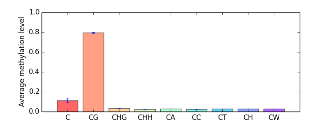
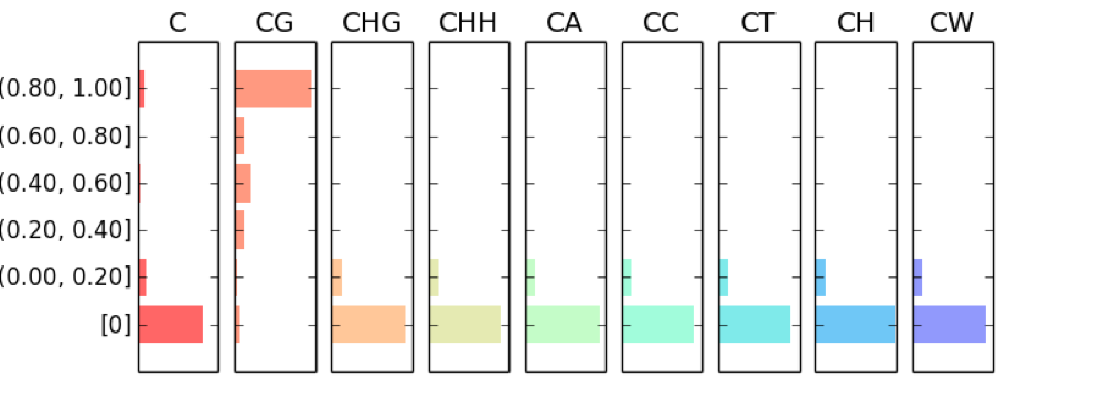
CGmapTools为全局DNA甲基化提供了丰富的统计分析。cgmaptools mstat命令将生成一个表和几个图，分别是：

mC contributions of different contexts in Pie chart
Bulk mC levels of different contexts
Fragmented distribution of mC in different contexts

所以！此命令适用于CGmap文件内包含不同种类的C context，如果CGmap文件只有CpG位点，那么这条命令可以不用跑了，除非重新生成CGmap。

5.8.1 命令

#   Usage: cgmaptools mstat [-i <CGmap>]  
#         (aka CGmapStatMeth)
#   Description: Generate the bulk methylation.
#   Contact:     Guo, Weilong; guoweilong@126.com
#   Last Update: 2018-05-02
#   Output Ex:
#      MethStat        context C       CG      CHG      CHH     CA      CC      CT      CH      CW
#      mean_mC         global  0.0798  0.3719  0.0465  0.0403  0.0891  0.0071  0.0241  0.0419  0.0559
#      sd_mCbyChr      global  0.0078  0.0341  0.0163  0.0110  0.0252  0.0049  0.0076  0.0096  0.0148
#      count_C         global  10000   1147    2332    6521    3090    2539    3224    8853    6314
#      contrib_mC      global  1.0000  0.5348  0.1360  0.3292  0.3452  0.0228  0.0973  0.4652  0.4424
#      quant_mC        [0]     8266    471     2012    5783    2422    2421    2952    7795    5374
#      quant_mC   (0.00 ,0.20] 705     182     155     368     272     97      154     523     426
#      mean_mC_byChr   chr1    0.0840  0.4181  0.0340  0.0412  0.0794  0.0065  0.0251  0.0393  0.0513
#      mean_mC_byChr   chr10   0.0917  0.4106  0.0758  0.0421  0.0968  0.0097  0.0349  0.0502  0.0655
#   
#   Options:
#     -h, --help            show this help message and exit
#     -i FILE               File name end with .CGmap or .CGmap.gz. If not
#                           specified, STDIN will be used.
#     -c COVERAGE           The minimum coverage for site selection [Default: 10]
#     -f FILE, --figure-type=FILE
#                           png, pdf, eps. Will not generate figure if not
#                           specified
#     -H FLOAT              Height of figure in inch [Default: 3]
#     -W FLOAT              Width of figure in inch [Default: 8]
#     -p STRING             Prefix for output figures
#     -t STRING, --title=STRING
#                           title in the output figures

Example

cgmaptools mstat -i WG.CGmap.gz -c 4 -f png -p WG -t WG > WG.mstat.data

Output format

Example

MethStat        context C       CG      CHG     CHH     CA      CC      CT      CH      CW
mean_mC         global  0.0798  0.3719  0.0465  0.0403  0.0891  0.0071  0.0241  0.0419  0.0559
sd_mCbyChr      global  0.0078  0.0341  0.0163  0.0110  0.0252  0.0049  0.0076  0.0096  0.0148
count_C         global  10000   1147    2332    6521    3090    2539    3224    8853    6314
contrib_mC      global  1.0000  0.5348  0.1360  0.3292  0.3452  0.0228  0.0973  0.4652  0.4424
quant_mC        [0]     8266    471     2012    5783    2422    2421    2952    7795    5374
quant_mC   (0.00 ,0.20] 705     182     155     368     272     97      154     523     426
mean_mC_byChr   chr1    0.0840  0.4181  0.0340  0.0412  0.0794  0.0065  0.0251  0.0393  0.0513
mean_mC_byChr   chr10   0.0917  0.4106  0.0758  0.0421  0.0968  0.0097  0.0349  0.0502  0.0655

Output figures

下面的三张图从左到右分别为：
Figure 5.9: mC contribution example
Figure 5.10: Bulk mC example
Figure 5.11: mC fragmented distribution example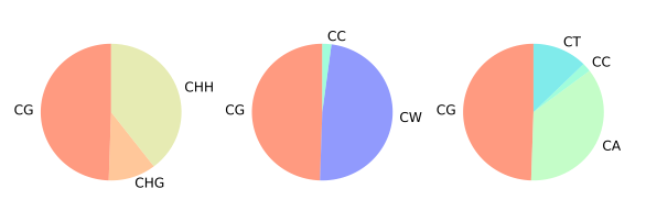

5.9 mtr

cgmaptools mtr命令将计算每个感兴趣区域的DNA甲基化水平。例如我们对基因组上的启动子感兴趣，可以把启动子区域的BED文件作为输入，计算每一个输入的启动子的甲基化水平。
Tips：虽然cgmaptools mtr不支持多样本同时运行，但是可以每个样本对同样的区域单独运行cgmaptools mtr，然后使用R等工具合并多样本的运行结果，获得多样本在区域内的甲基化水平矩阵。但是得注意，因为每个样本检测到的位点数目不尽相同，所以即使是同一个组别的样本，有可能在一个promoter上的甲基化水平差异也很大，这种情况就可以想办法进行过滤或处理。

5.9.1 命令

#   Usage: cgmaptools mtr [-i <CGmap>] -r <region> [-o <output>]
#         (aka CGmapToRegion)
#   Description: Calculated the methylation levels in regions in two ways.
#   Format of Region file:
#     #chr    start_pos  end_pos
#      chr1   8275       8429
#   Output file format:
#      #chr  start_pos  end_pos  mean(mC)  #_C  #read(C)/#read(T+C)  #read(T+C)
#      chr1   8275       8429     0.34     72         0.40             164
#   Note: The two input CGmap files should be sorted by Sort_chr_pos.py first.
#         This script would not distinguish CG/CHG/CHH contexts.
#   
#   Options:
#     -h, --help  show this help message and exit
#     -i FILE     File name end with .CGmap or .CGmap.gz. If not specified, STDIN
#                 will be used.
#     -r FILE     Filename for region file, support *.gz
#     -o OUTFILE  To standard output if not specified.

Example

cgmaptools mtr -i WG.CGmap.gz -r region.bed -o WG.mtr.gz

Input region format

#chr    start_pos  end_pos
chr1    8275       8429

Output format

Example

chr1   8275   8429    0.34   72    0.40   164
chr1   8899   8999    0.20   40    0.33   198
chr2   8275   8429    0.50   12    0.45   40

Column Description

Figure 5.12: Output format description for cgmaptools mtr

DNA 甲基化数据分析工具和数据库

cgmaptools综合分析BS-seq

背景知识

逐个功能讲解

4 SNV calling

5 Methylation Analysis

5.1 dms

5.2 dmr

cgmaptools merge

5.3 asm

5.4 mbed

5.5 mbin

5.6 mmbin （multi mbin）

5.7 mfg(meth fragmented)

5.8 mstat

5.9 mtr