希望每个学徒和实习生都可以在生信技能树的舞台上大放光彩！

下面是 “YuYuFiSH” 的分享

现在有很多方法将甲基化和生物学调节活性联合起来分析，例如：联合显著甲基化位点和附近基因表达，或者探索差异甲基化区域的 TF 富集等等。但是这些都依赖于阈值的选取，先提取出差异位点，并没有充分利用全基因组数据。另外，研究表明，还有其他因素影响甲基化水平，如位点周边甲基化图谱形状。

所以，作者开发了一种新的计算方法，利用全基因组甲基化水平评估生物学调节活性

MIRA (Methylation-based Inference of Regulatory Activity)

↓

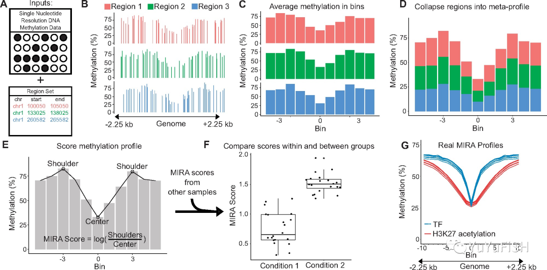
A：两种输入数据：

• 样本的 DNA 甲基化数据（(WGBS or RRBS or microarrays）
• 一组共享生物学注释的基因组区域集（ChIP-seq, DNase-seq, or ATAC-seq or large-scale genomics projects like LOLA R packages）

B：首先为 4.5 kb 区域绘制对应 CpG 位点的 DNA 甲基化水平

C：将每个区域分成 11 个大小大致相等的 bin，并根据对应 CpG 位点计算平均甲基化水平

D：将所有区域聚合成单个 DNA 甲基化图谱

E：通过公式求出 MIRA score

F：可以对不同状态的样本 MIRA score 进行比较（注意：样本间均使用相同的基因组区域，分数的显著差异表明该区域集的调节活性存在差异 differential activity of this region set）

G：例如，此图是来源于文章六个间充质干细胞样品的 DNA 甲基化数据的 TF 区域集和 H3K27 乙酰化区域的 MIRA 图

下面介绍下基本用法

• 简化甲基化测序（Reduced Representation Bisulfite Sequencing，RRBS）
• 12 个尤文肉瘤样本 Ewing sarcoma samples
• 12 个肌肉样本 myotube (muscle) samples
• 两组特定的 DHSs 区域
• one with Ewing-specific DHSs
• a one with muscle-specific DHSs

（来源：Regulatory Elements Database (databio.org)）

• 下载链接：

http://cloud.databio.org/vignettes/MIRA_Ewing_Vignette_Files.tar.gz

早在 20 世纪 80 年代初期，研究人员发现染色质对脱氧核糖核酸酶 I(DNase I) 的敏感性与基因的转录有关，即当一个基因处于转录活性状态时，含有这个基因的染色质区域对 DNase I 降解的敏感性要比无转录活性区域高出 100 倍以上，被称为 DNase I 超敏感位点（DNase I hypersensitive site，DHS）

`options(stringsAsFactors = F)
BiocManager::install(‘MIRA’)
# install.packages(“path/to/MIRA/directory”, repos=NULL, type=”source”)
# devtools::install_github(“databio/MIRA”)

library(MIRA)
library(data.table) # for the functions: fread, setkey, merge
library(GenomicRanges) # for the functions: GRanges, resize
library(ggplot2) # for the function: ylab

data input
# 12 Ewing samples: T1-T12
pathToData <- “MIRAEwing_Vignette_Files/MIRA_Ewing_Vignette_Files/“
ewingFiles <- paste0(pathToData, “EWS_T”, 1:12, “.bed”)
# 12 muscle related samples, 3 of each type
muscleFiles <- c(“Hsmm“,”Hsmmt“,”Hsmmfshd“,”Hsmmtubefshd_”)
muscleFiles <- paste0(pathToData, muscleFiles, rep(1:3, each=4), “.bed”)
RRBSFiles <- c(ewingFiles, muscleFiles)
# 2 region
regionSetFiles <- paste0(pathToData, c(“sknmc_specific.bed”, “muscle_specific.bed”))

`

3.1 甲基化文件：BSDTList

`BSDTList <- lapply(X=RRBSFiles, FUN=BSreadBiSeq)
class(BSDTList) #[1] “list”
BSDTList[1]

命名
names(BSDTList) <- tools::file_path_sans_ext(basename(RRBSFiles))
names(BSDTList)[1] # “EWS_T1”

`

`> class(BSDTList)
[1] “list”

BSDTList[1]
$EWS_T1
chr start methylCount coverage
1: chr1 10497 13 13
2: chr1 10525 13 13
3: chr1 10542 28 28
4: chr1 10563 16 17
5: chr1 10571 17 17
—-
4057237: chrY 56886884 1 1
4057238: chrY 56886894 1 1
4057239: chrY 56886917 1 1
4057240: chrY 56887089 31 42
4057241: chrY 56887099 36 42
`

每一行是一个甲基化位点

start (the coordinate of the C of the CpG)

methylCount (number of methylated reads)

coverage (total number of reads covering this site)

3.2 区域集文件：regionSets

regionSets <- lapply(X=regionSetFiles, FUN=fread) regionSets[1]

> regionSets[1] [[1]] V1 V2 V3 1: chr1 7853460 7853610 2: chr1 7857100 7857250 3: chr1 8067320 8067470 4: chr1 8606861 8607011 5: chr1 8821781 8821931 --- 5766: chrX 139981201 139981351 5767: chrX 144809119 144809269 5768: chrX 146967402 146967552 5769: chrX 151866668 151866818 5770: chrX 153238853 153239003

列明标注上染色体，起点，终点

转换成 GRanges 格式

regionSets <- lapply(X=regionSets, FUN=function(x) setNames(x, c("chr", "start", "end"))) regionSets <- lapply(X=regionSets, FUN= function(x) GRanges(seqnames=x$chr, ranges=IRanges(x$start, x$end)))

> regionSets[1] [[1]] GRanges object with 5770 ranges and 0 metadata columns: seqnames ranges strand <Rle> <IRanges> <Rle> [1] chr1 7853460-7853610 * [2] chr1 7857100-7857250 * [3] chr1 8067320-8067470 * [4] chr1 8606861-8607011 * [5] chr1 8821781-8821931 * ... ... ... ... [5766] chrX 139981201-139981351 * [5767] chrX 144809119-144809269 * [5768] chrX 146967402-146967552 * [5769] chrX 151866668-151866818 * [5770] chrX 153238853-153239003 * ------- seqinfo: 23 sequences from an unspecified genome; no seqlengths

上面核心原理也说到

MIRA scores 主要是基于区域集两端的甲基化水平和中心点求出

MIRA scores are based on the difference between methylation surrounding the regions versus the methylation at the region itself

所以，区域集长度选择很重要

这里区域的平均长度为 151，按照需求合理进行扩展长度到 5000bp（ resize）

`mean(width(regionSets[[1]]))
# [1] 151.4494

regionSets[[1]] <- resize(regionSets[[1]], 5000, fix=”center”)
regionSets[[2]] <- resize(regionSets[[2]], 5000, fix=”center”)
names(regionSets) <- c(“Ewing_Specific”, “Muscle_Specific”)
mean(width(regionSets[[1]])) # 5000
head(regionSets[[1]])

`

> head(regionSets[[1]]) GRanges object with 6 ranges and 0 metadata columns: seqnames ranges strand <Rle> <IRanges> <Rle> [1] chr1 7851035-7856034 * [2] chr1 7854675-7859674 * [3] chr1 8064895-8069894 * [4] chr1 8604436-8609435 * [5] chr1 8819356-8824355 * [6] chr1 10586298-10591297 * ------- seqinfo: 23 sequences from an unspecified genome; no seqlengths

接下来

就是把区域划分成大小大致相等的 bin，并根据对应 CpG 位点计算平均甲基化水平，再聚合成单个 DNA 甲基化图谱

# 挑其中 6 个样本分析 subBSDTList <- BSDTList[c(1, 5, 9, 13, 17, 21)] bigBin <- lapply(X=subBSDTList, # 甲基化水平 FUN=aggregateMethyl, # 算法函数 GRList=regionSets, # 区域文件 binNum=21, # bin 数量 minBaseCovPerBin=0)

可以调节两个参数

binNum ：bin 的数量，会影响到结果的分辨率与噪声（数量越多，分辨率越高，导致每个 bin 越小，包含更少的 read，噪声越高）

minBaseCovPerBin：每个 bin 的最小覆盖率（只用纳入的甲基化文件有 coverage）

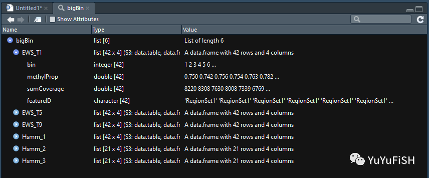
# 增加样本名并转换成 data frame bigBinDT1 <- rbindNamedList(bigBin, newColName = "sampleName") dim(bigBinDT1) # 252 5 head(bigBinDT1)

> head(bigBinDT1) bin methylProp sumCoverage featureID sampleName 1: 1 0.7502673 8219.5 Ewing_Specific EWS_T1 2: 2 0.7417109 8308.5 Ewing_Specific EWS_T1 3: 3 0.7559284 7629.5 Ewing_Specific EWS_T1 4: 4 0.7537173 8007.5 Ewing_Specific EWS_T1 5: 5 0.7625003 7339.0 Ewing_Specific EWS_T1 6: 6 0.7821055 6769.0 Ewing_Specific EWS_T1

可以看到新增了一列 methylProp

（ methylProp = methylCount/coverage ）

最后针对结果 bigBinDT1 增加样本分组信息

`exampleAnnoDT2 <- fread(system.file(“extdata”, “exampleAnnoDT2.txt”,
package=”MIRA”))
setkey(exampleAnnoDT2, sampleName)
setkey(bigBinDT1, sampleName)
head(exampleAnnoDT2)

bigBinDT1 <- merge(bigBinDT1, exampleAnnoDT2, all.x=TRUE)
head(bigBinDT1)

`

新增一列 sampleType

`> head(exampleAnnoDT2)
sampleName sampleType
1: EWS_T1 Ewing
2: EWS_T10 Ewing
3: EWS_T11 Ewing
4: EWS_T12 Ewing
5: EWS_T2 Ewing
6: EWS_T3 Ewing

head(bigBinDT1)
sampleName bin methylProp sumCoverage featureID
1: EWS_T1 1 0.7502673 8219.5 RegionSet1
2: EWS_T1 2 0.7417109 8308.5 RegionSet1
3: EWS_T1 3 0.7559284 7629.5 RegionSet1
4: EWS_T1 4 0.7537173 8007.5 RegionSet1
5: EWS_T1 5 0.7625003 7339.0 RegionSet1
6: EWS_T1 6 0.7821055 6769.0 RegionSet1
sampleType
1: Ewing
2: Ewing
3: Ewing
4: Ewing
5: Ewing
6: Ewing
table(bigBinDT1$sampleType)

Ewing Muscle-related
126 84

`

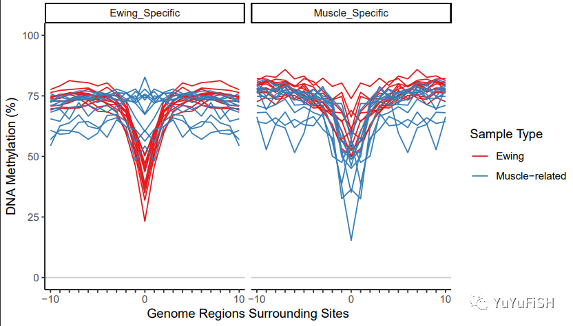
plotMIRAProfiles(binnedRegDT=bigBinDT1)

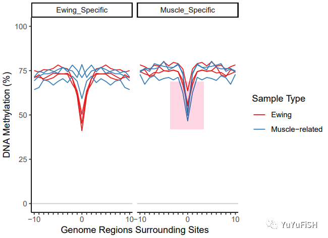
初步看一下甲基化曲线

作者认为，在查看肌肉特定区域集时，对于肌肉相关样品来说，下降的宽度太窄，MIRA 中的评分函数可能会遇到问题，因为最好跌幅至少跨越 5 个 bin

针对这个结果，我们可以对应调整区域大小，但也不应减少太多，如果区域太小，则可能会有更多的噪声

重新调整再跑一遍上面步骤

`regionSets[[1]] <- resize(regionSets[[1]], 4000, fix=”center”) # Ewing
regionSets[[2]] <- resize(regionSets[[2]], 1750, fix=”center”) # muscle

bigBin <- lapply(X=BSDTList, FUN=aggregateMethyl, GRList=regionSets,
binNum=21, minBaseCovPerBin=0)
bigBinDT2 <- rbindNamedList(bigBin)

data.table functions are used to add info from annotation object to bigBinDT2
setkey(exampleAnnoDT2, sampleName)
setkey(bigBinDT2, sampleName)
bigBinDT2 <- merge(bigBinDT2, exampleAnnoDT2, all.x=TRUE)
plotMIRAProfiles(binnedRegDT=bigBinDT2)

`

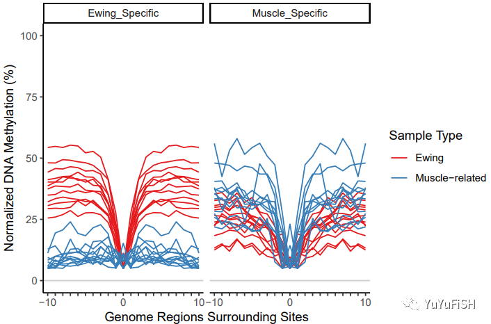
现在曲线看起来更好了

通过减去最小的 methylProp 进行归一化

使 MIRA 评分更多地与轮廓的形状有关，而与平均甲基化的关系较少

bigBinDT2[, methylProp := methylProp - min(methylProp) + .05, by=.(featureID, sampleName)] normPlot <- plotMIRAProfiles(binnedRegDT=bigBinDT2) normPlot + ylab("Normalized DNA Methylation (%)")

sampleScores <- calcMIRAScore(bigBinDT2, shoulderShift="auto", regionSetIDColName="featureID", sampleIDColName="sampleName") head(sampleScores) # featureID sampleName score # 1: Ewing_Specific EWS_T1 2.180698 # 2: Ewing_Specific EWS_T10 2.114649 # 3: Ewing_Specific EWS_T11 2.064900 # 4: Ewing_Specific EWS_T12 2.290313 # 5: Ewing_Specific EWS_T2 1.987881 # 6: Ewing_Specific EWS_T3 2.230074

重新加入分组信息，并做出箱式图

`setkey(exampleAnnoDT2, sampleName)
setkey(sampleScores, sampleName)
sampleScores <- merge(sampleScores, exampleAnnoDT2, all.x=TRUE)

plotMIRAScores(sampleScores)

`

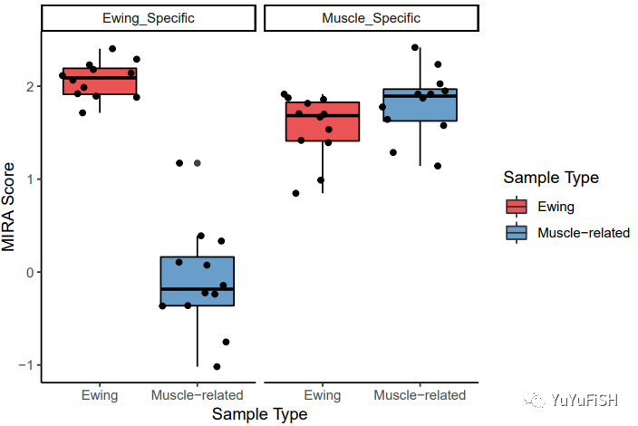
分别对两个区域进行 the Wilcoxon rank sum test 非参数分析

• the Ewing-specific region set

EwingSampleEwingRegions <- sampleScores[sampleScores$sampleType == "Ewing" & sampleScores$featureID == "Ewing_Specific", ] myoSampleEwingRegions <- sampleScores[sampleScores$sampleType == "Muscle-related" & sampleScores$featureID == "Ewing_Specific", ] wilcox.test(EwingSampleEwingRegions$score, myoSampleEwingRegions$score) # Wilcoxon rank sum test # # data: EwingSampleEwingRegions$score and myoSampleEwingRegions$score # W = 144, p-value = 7.396e-07 # alternative hypothesis: true location shift is not equal to 0

• the muscle-specific region set

EwingSampleMyoRegions <- sampleScores[sampleScores$sampleType == "Ewing" & sampleScores$featureID == "Muscle_Specific", ] myoSampleMyoRegions <- sampleScores[sampleScores$sampleType == "Muscle-related" & sampleScores$featureID == "Muscle_Specific", ] wilcox.test(EwingSampleMyoRegions$score, myoSampleMyoRegions$score) # Wilcoxon rank sum test # # data: EwingSampleMyoRegions$score and myoSampleMyoRegions$score # W = 40, p-value = 0.06836 # alternative hypothesis: true location shift is not equal to 0

正如预期的那样，我们发现在其尤因肉瘤特定 DHS 中，两种样本的 MIRA 评分差异具有统计学意义，且尤因肉瘤样本的评分更高，意味着在该区域中有更高的调节活性

1. 该算法最终得到的生物学意义关键在于纳入的甲基化文件和感兴趣的基因区域
2. 作者发现 MIRA 分数也可以推断转录因子的调节活性，但只是间接推断
3. 因为甲基化谱可能受到除感兴趣 TF 以外的其他 TF 的影响。因此，一个样本在 TF 结合区域的 MIRA 评分可能高于另一个样本，但对该 TF 的活性仍然较低
4. 或者得分较高的样本通常与获得区域集的样本具有更相似的染色质状态（例如，当在来自多种组织 / 细胞类型的样品上使用 MIRA 时，并且区域集来自与某些但不是全部样品相同的组织 / 细胞类型）

🍥Multimodal analysis of cell-free DNA whole-genome sequencing for pediatric cancers with low mutational burden

Nature Communications IF=14.9 2021

🍥Multiomic Analysis Reveals Comprehensive Tumor Heterogeneity and Distinct Immune Subtypes in Multifocal Intrahepatic Cholangiocarcinoma

Clinical Cancer Research IF=12.5 2021

末友情宣传

强烈建议你推荐给身边的博士后以及年轻生物学 PI，多一点数据认知，让他们的科研上一个台阶：

• 数据挖掘（GEO,TCGA, 单细胞）2022 年 5 月场，快速了解一些生物信息学应用图表
• 生信入门课 - 2022 年 5 月场，你的生物信息学第一课

参考：

[1] MIRA: an R package for DNA methylation-based inference of regulatory activity | Bioinformatics | Oxford Academic (oup.com)

https://academic.oup.com/bioinformatics/article/34/15/2649/4916061

[2] Methylation-Based Inference of Regulatory Activity • MIRA (databio.org)

https://code.databio.org/MIRA/index.html

[3]MIRA: Methylation-Based Inference of Regulatory Activity (bioconductor.org)

http://bioconductor.org/packages/release/bioc/manuals/MIRA/man/MIRA.pdf

[4]Getting Started with Methylation-based Inference of Regulatory Activity (bioconductor.org)

https://bioconductor.org/packages/devel/bioc/vignettes/MIRA/inst/doc/GettingStarted.html
https://mp.weixin.qq.com/s/iGXLEW13SFcVGBP8ytvVPg