摘抄于:https://www.jianshu.com/p/2773231dfc0f
- Tutorial: Normalization of BigWig files using TMM from edgeR
- Tutorial: Using EnrichedHeatmap for visualization of NGS experiments
- 绘图示例数据链接
#### A minimal example on how to use EnrichedHeatmap together with rtracklayer:require(EnrichedHeatmap)require(rtracklayer)require(circlize)require(data.table)## We start from a BED file with coordinates and load as GRanges:tmp.targets <- makeGRangesFromDataFrame(df = fread("~/your.bed", header = F),seqnames.field = "V1", start.field = "V2", end.field = "V3")## Say we want to take the peak center and extend it by 5kb in each direction:tmp.extension <- 5000## Extend center of the peaks by tmp.extension in each direction:tmp.targets_extended <- resize(tmp.targets, fix = "center", width = tmp.extension*2)## Now load the content of the bigwig limited to the regions we are interested in.## This is much quicker than loading the entire bigwig and does not consume so much memory:tmp.bigwig <- rtracklayer::import("~/your.bigwig" ,format = "BigWig",selection = BigWigSelection(tmp.targets_extended))## create the normalizedMatrix that EnrichedHeatmap accepts as input.## We use the tmp.targets center (width=1) because from what I understand normalizeMatrix## does not allow to turn off its extend= option. Therefore we trick it by simply## providing the peak centers and then let the function extend it by our predefined window size.normMatrix <- normalizeToMatrix(signal = tmp.bigwig,target = resize(tmp.targets, fix = "center", width = 1),background = 0,keep = c(0, 0.99), ## minimal value to the 99th percentiletarget_ratio = 0,mean_mode = "w0", ## see ?EnrichedHeatmap on other optionsvalue_column = "score", ## = the name of the 4th column of the bigwigextend = tmp.extension)## a color gradient that I personally find visually appealing, which will cover## the range from the lowest value of normMatrix to the 99th percentile## (99th perc. avoids extreme values skewing the heatmap):col_fun = circlize::colorRamp2(quantile(normMatrix, c(0, .99)), c("darkblue", "darkgoldenrod1"))## heatmap function:enrHtmp <- EnrichedHeatmap( mat = normMatrix,pos_line = FALSE, ## no dashed lines around the startborder = FALSE, ## no box around heatmapcol = col_fun, ## color gradients from abovecolumn_title = "Nice Heatmap", ## column titlecolumn_title_gp = gpar(fontsize = 15, fontfamily = "sans"),## these three options produce a high-quality pdf## while keeping the file size small so that it easily fits## nto any powerpoint presentation without crashing ituse_raster = TRUE, raster_quality = 10, raster_device = "png",## turn off background colorsrect_gp = gpar(col = "transparent"),## legend:heatmap_legend_param = list(legend_direction = "horizontal", ## legend horizontaltitle = "legend_title"),## options for the profile plot on toptop_annotation = HeatmapAnnotation(enriched = anno_enriched(gp = gpar(col = "black", lty = 1, lwd=2),col="black"))) ## end of EnrichedHeatmap function## Instead of plotting to the Rstudio device save as pdf,## with width-2 and height-6 I personally find the heatmap visually most appealing,## it looks good while not being too "fat":pdf("~/EnrichedHeatmap.pdf", width = 2, height = 6)## Plot it:draw(enrHtmp, ## plot the heatmap from aboveheatmap_legend_side = "bottom", ## we want the legend below the heatmapannotation_legend_side = "bottom", ##padding = unit(c(4, 4, 4, 4), "mm") ## some padding to avoid labels beyond plot borders)dev.off() ## close the pdf
出图示例: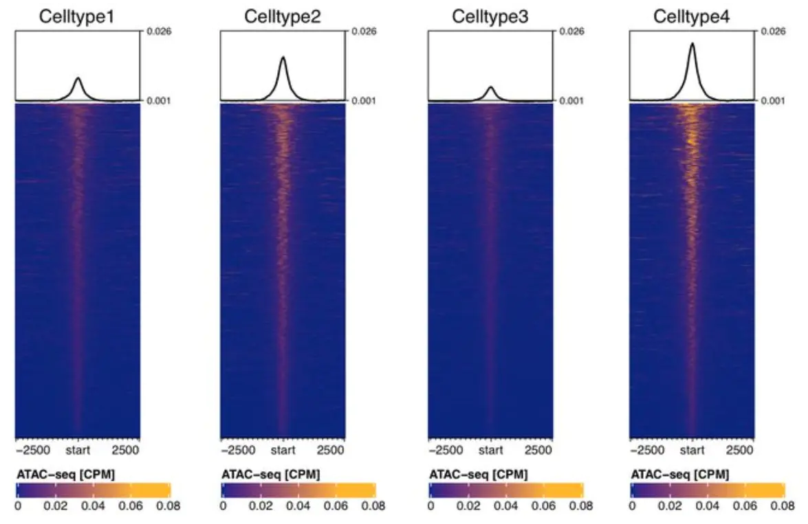

若有收获,就点个赞吧
0 人点赞
