0.4772018.05.07 16:07:08 字数 3,440 阅读 11,718

参考：https://bioconductor.org/packages/release/bioc/vignettes/ChAMP/inst/doc/ChAMP.html
http://blog.csdn.net/joshua_hit/article/details/54982018
https://www.jianshu.com/p/6411e8acfab3

ChAMP package 是用来分析 illuminate 甲基化数据的包 (EPIC and 450k)。

包括：

• 不同格式的数据导入 (e.g. from .idat files or a beta-valued matrix)
• Quality Control plots
• Type-2 探针的矫正方法：SWAN1, Peak Based Correction (PBC)2 and BMIQ3 (the default choice).
• The popular Functional Normalization function offered by the minfi package is also available.
• 查看批次效应的方法：singular value decomposition (SVD) method，for correction of multiple batch effects the ComBat method
• 通过 RefbaseEWAS 矫正 cell-type heterogeneity
• 也可以推断 CNV 变异
• Differentially Methylated Regions (DMR) （Lasso method，Bumphunter and DMRcate）
• find Differentially Methylated Blocks
• Gene Set Enrichment Analysis (GSEA)
• infer gene modules in user-specified gene-networks that exhibit differential methylation between phenotypes （整合 FEM package）
• 其他分析甲基化数据的包：(including IMA, minfi, methylumi, RnBeads and wateRmelon)

1、安装 ChAMP 包:

source("https://bioconductor.org/biocLite.R")
biocLite("ChAMP")
#或者直接安装依赖包
source("http://bioconductor.org/biocLite.R")
biocLite(c("minfi","ChAMPdata","Illumina450ProbeVariants.db","sva","IlluminaHumanMethylation450kmanifest","limma"))
#如果报错，试用
biocLite("YourErrorPackage")
#最后加载包
library("ChAMP")
如果报错：
错误: package or namespace load failed for 'ChAMP' in inDL(x, as.logical(local), as.logical(now), ...):
 无法载入共享目标对象‘D:/work/R-3.4.3/library/mvtnorm/libs/x64/mvtnorm.dll’：:
  `已达到了DLL数目的上限...
解决方案就是设置环境变量R_MAX_NUM_DLLS, 不管是什么操作系统，R语言对应的环境变量都可以在.Renviron文件中进行设置。
这个文件可以保存在任意目录下，文件中就一句话，内容如下
R_MAX_NUM_DLLS=500
500表示允许的最多的dll文件数目，设置好之后，重新启动R, 然后输入如下命令
normalizePath("d:/Documents/.Renviron", mustWork = FALSE)
第一个参数为.Renviron文件的真实路径，然后在加载ChAMP包就可以了

2、用测试数据跑流程

测试数据包括 450k(.idat) 和 850k（simulated EPIC data）两个数据集

#450k数据集包括8个样本的肺癌数据，4个肿瘤组织（T）和4个对照（C）
testDir=system.file("extdata",package="ChAMPdata")
myLoad <- champ.load(testDir,arraytype="450K")
#850k数据集包括16个样本，但是都是由一个样本修改DMP 和 DMR而来。
data(EPICSimData)

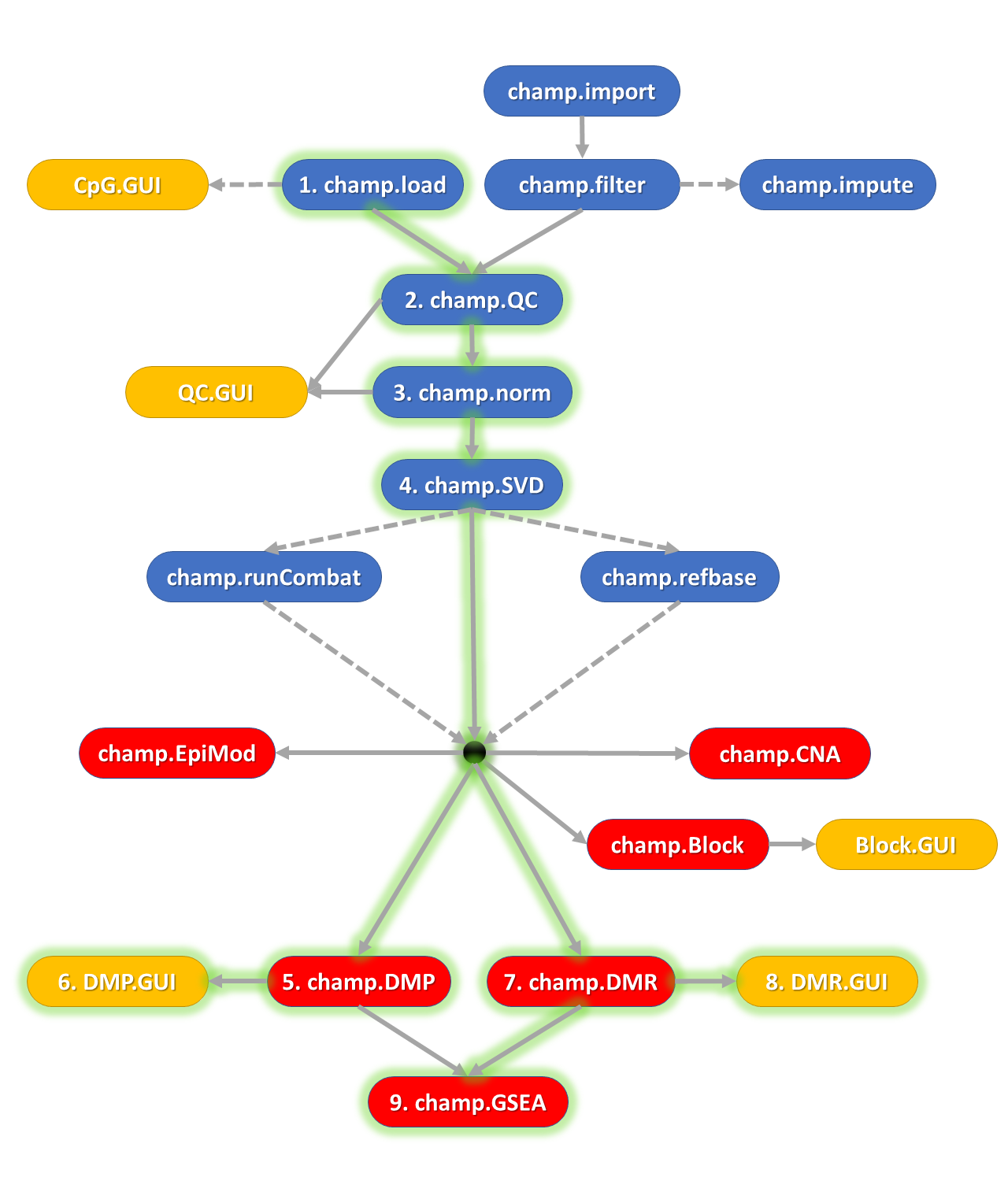
3、ChAMP Pipeline

untitled.png

绿色发光线表示主要的分析步骤，灰色为可选的步骤。黑点表示准备好的甲基化数据。
蓝色表示准备工作，比如 Loading, Normalization, Quality Control checks etc.
红色表示产生分析结果：Differentially Methylated Positions (DMPs), Differentially Methylated Regions (DMRs), Differentially methylated Blocks, EpiMod (a method for detecting differentially methylated gene modules derived from FEM package), Pathway Enrichment Results etc.
黄色表示交互界面画图

• 450k 步骤
• Full Pipeline
  #一步跑完结果，但是可能报错
  champ.process(directory = testDir)

• 一步一步跑
  myLoad <- cham.load(testDir)
  CpG.GUI()
  champ.QC() # Alternatively: QC.GUI()
  myNorm <- champ.norm()
  champ.SVD()
  myDMP <- champ.DMP()
  DMP.GUI()
  myDMR <- champ.DMR()
  DMR.GUI()
  myBlock <- champ.Block()
  Block.GUI()
  myGSEA <- champ.GSEA()
  myEpiMod <- champ.EpiMod()
  myCNA <- champ.CNA()
  myRefbase <- champ.refbase()

  Or you may separate about code as champ.import(testDir) + champ.filter()

  If Batch detected, run champ.runCombat() here.

  If DataSet is Blood samples, run champ.refbase() here.

• EPIC pipeline
  data(EPICSimData)
  CpG.GUI(arraytype=”EPIC”)
  champ.QC() # Alternatively QC.GUI(arraytype=”EPIC”)
  myNorm <- champ.norm(arraytype=”EPIC”)
  champ.SVD()
  myDMP <- champ.DMP(arraytype=”EPIC”)
  DMP.GUI()
  myDMR <- champ.DMR()
  DMR.GUI()
  myDMR <- champ.DMR(arraytype=”EPIC”)
  DMR.GUI(arraytype=”EPIC”)
  myBlock <- champ.Block(arraytype=”EPIC”)
  Block.GUI(arraytype=”EPIC”) # For this simulation data, not Differential Methylation Block is detected.
  myGSEA <- champ.GSEA(arraytype=”EPIC”)
  myEpiMod <- champ.EpiMod(arraytype=”EPIC”)
  

  myLoad <- champ.load(directory = testDir,arraytype=”EPIC”)

  We simulated EPIC data from beta value instead of .idat file,

  but user may use above code to read .idat files directly.

  Here we we started with myLoad.

  If Batch detected, run champ.runCombat() here.This data is not suitable.

  champ.CNA(arraytype=”EPIC”)

  champ.CNA() function call for intensity data, which is not included in our Simulation data.

最多在 8G 内存电脑上可以跑 200 个样本，如果在服务器上多核跑，需要命令

library("doParallel")
detectCores()

Description of ChAMP Pipelines

6.1 Loading Data

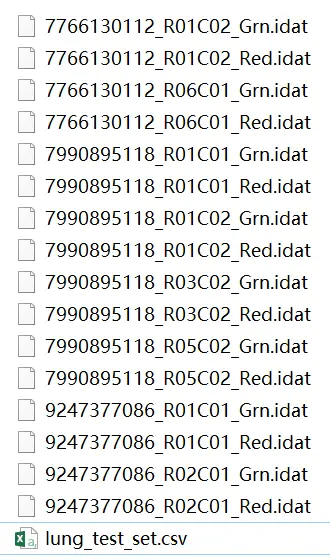
image.png

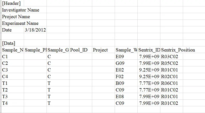
image.png

.idat files 为原始芯片文件，包括 pd file (Sample_Sheet.csv) 文件（表型，编号等）

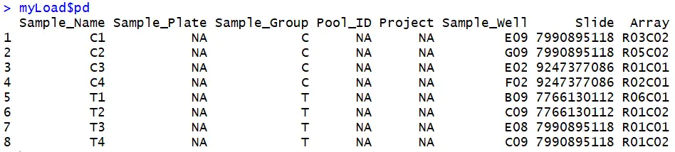
image.png

#以450k数据作为演示：
#首先看下pd数据，有时候不同的实验格式不一致
myLoad$pd
#发现Sample_Group栏C代表control,T代表Tumor。有的可能用“Diagnose” or “CancerType”等代替

6.2 Filtering Data

• ChAMP 提供了 champ.filter() 函数，可以输入 (beta, M, Meth, UnMeth, intensity) 格式的文件并进行过滤质控。 新版本的 ChAMP 包中 champ.load() 函数已经包含了此功能。
• champ.filter() 函数有个参数 autoimpute，可以填补或保留由过滤导致的 NA 空缺值。
• 如果输入多个数据框进行过滤，他们的行名和列名必须一致，否则 champ.filter() 认为是不同来源的数据，将停止过滤。
• 低质量的样本（有较多的探针没有信号）将会被过滤掉，Sample_Name 要与 pd file 中的列名称一致。
• imputation 需要 detection P matrix, beta or M matrix 信息，且 ProbeCutoff 不能等于 0，这个参数控制探针的 NA ratio，来决定是否填补。
• 如果想用 beadcount 信息进行过滤，champ.import() 函数会返回 beads 信息。
  使用方法为：
  myImport <- champ.import(testDir)
  myLoad <- champ.filter()
  #与champ.load()函数功能一致
  Section 1: Read PD Files Start： Reading CSV File
  Section 2: Read IDAT files Start：Extract Mean value for Green and Red Channel Success
  Your Red Green Channel contains 622399 probes.
  Section 3: Use Annotation Start：Reading 450K Annotation，there are 613 control probes in Annotation，Generating Meth and UnMeth Matrix，485512 Meth probes
  Generating beta Matrix
  Generating M Matrix
  Generating intensity Matrix
  Calculating Detect P value
  Counting Beads
  You may want to process champ.filter() next，This function is provided for user need to do filtering on some beta (or M) matrix, which contained most filtering system in champ.load except beadcount.
  #过滤步骤
  Section 1: Check Input Start：You have inputed beta,intensity for Analysis.
  Checking Finished :filterDetP,filterBeads,filterMultiHit,filterSNPs,filterNoCG,filterXY would be done on beta,intensity.
  You also provided :detP,beadcount .
  Section 2: Filtering Start
  The fraction of failed positions per sample
  Failed CpG Fraction.
  C1 0.0013429122
  C2 0.0022162171
  C3 0.0003563249
  C4 0.0002842360
  T1 0.0003831007
  T2 0.0011946152
  T3 0.0014953286
  T4 0.0015447610
  Filtering probes with a detection p-value above 0.01.
  Removing 2728 probes.
  Filtering BeadCount Start
  Filtering probes with a beadcount <3 in at least 5% of samples.
  Removing 9291 probes
  Filtering NoCG Start
  Only Keep CpGs, removing 2959 probes from the analysis.
  Filtering SNPs Start
  Using general 450K SNP list for filtering.
  Filtering probes with SNPs as identified in Zhou’s Nucleic Acids Research Paper 2016.
  Removing 49231 probes from the analysis.
  Filtering MultiHit Start
  Filtering probes that align to multiple locations as identified in Nordlund et al
  Removing 7003 probes from the analysis.
  Filtering XY Start
  Filtering probes located on X,Y chromosome, removing 9917 probes from the analysis.
  Updating PD file
  Fixing Outliers Start
  Replacing all value smaller/equal to 0 with smallest positive value.
  Replacing all value greater/equal to 1 with largest value below 1..

  champ.load()具体步骤为：

  导入之后可以用champ.filter() 函数进行过滤

过滤步骤为：

• detection p-value (<0.01)。这个值储存在. idat 文件中，champ.import() 函数读入这个值并形成数据框。p< 0.01 的探针认为实验失败。过滤过程为：样本探针失败率阈值 = 0.1，再在剩下的样本中过滤探针。参数 SampleCutoff 和 ProbeCutoff 控制这两个阈值。
• ChAMP will filter out probes with <3 beads ( filterBeads 参数控制) in at least 5% （beadCutoff 参数控制）of samples per probe.
• 默认过滤 non-CpG probes
• by default ChAMP will filter all SNP-related probe。需要用 population 参数选择群体。如果不选，用 General Recommended Probes provided by Zhou to do filtering。
• ChAMP will filter all multi-hit probes.
• 默认过滤掉 chromosome X and Y 上的探针。filterXY 参数控制。
  如果没有原始的. IDAT 数据，用 champ.filter() 函数进行过滤。

注意：

champ.load() can not perform filtering on beta matrix alone. For users have no .IDAT data but beta matrix and Sample_Sheet.csv, you may want perform filtering using the champ.filter() function and then use following functions to do analysis.

CpG.GUI() 函数查看甲基化位点的分布情况。CpGs on chromosome, CpG island, TSS reagions.

# 在分析中的任何位置都可用这个函数，
CpG.GUI(CpG=rownames(myLoad$beta),arraytype="450K")
#注意用的beta值，任何时候用beta值都可以，比如看DMP的情况

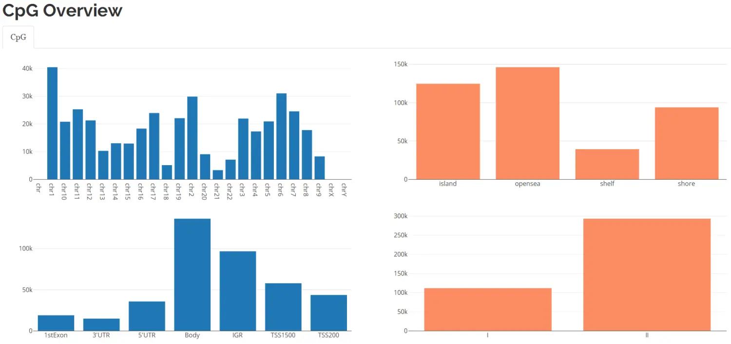
image.png

6.3 Further quality control and exploratory analysis

用 champ.QC() function and QC.GUI() function 检查数据质量

champ.QC() 函数会生成三个图：

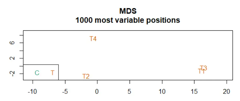
image.png

mdsPlot (Multidimensional Scaling Plot): 基于前 1000 个最易变化的位点查看样本的相似度，用颜色标记不同的样本分组。

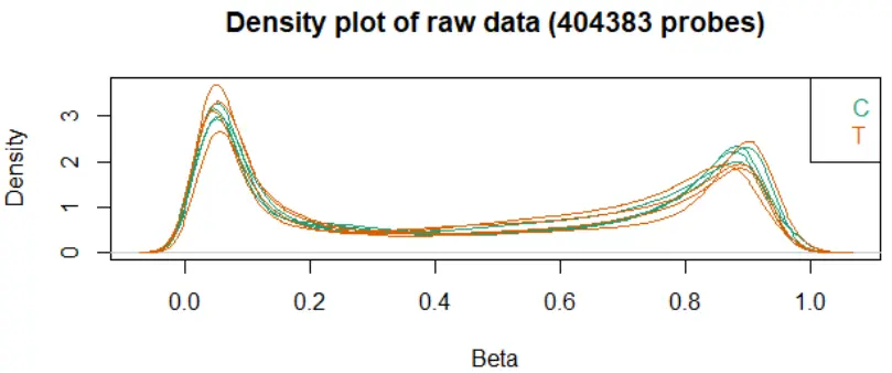
image.png

densityPlot: 查看每个样本的 beta 值分布，有严重偏离的样本预示着质量较差（如亚硫酸盐处理不完全等）

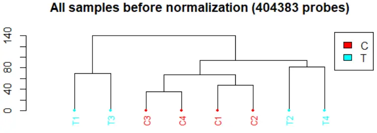
image.png

dendrogram: 所有样本的聚类图。champ.QC() 函数中 Feature.sel=”None” 参数表示直接通过探针数值来计算样本的距离，比较耗内存；还有 “SVD” method。

QC.GUI() 函数也可以画图，但是比较耗内存。
包括 5 张图：mdsPlot, type-I&II densityPlot, sample beta distribution plot, dendrogram plot and top 1000 most variable CpG’s heatmap.

QC.GUI(beta=myLoad$beta,arraytype="450K")

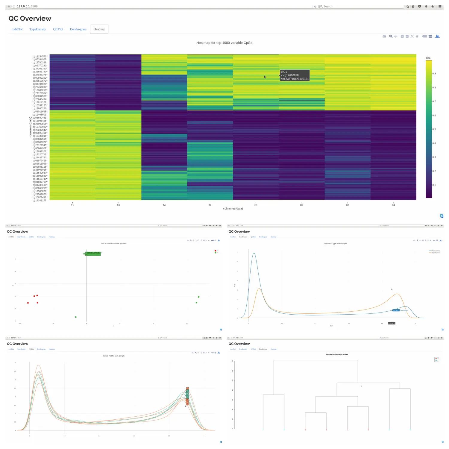
image.png

• type-I&II densityPlot 图可以帮助查看两个探针的标准化状态。
• Top variable CpGs’ heatmap 将前 1000 个差异最大的位点和状态表示出来。

6.4 Normalization

type-I 和 type-II 两种探针化学反应不同，设计也不同，导致分布区域也不同。这两种探针检测出的差异可能是因为探针所在位置不平衡导致的生物学差异引起的（如 CpG 位置的差异引起的）。最主要是 type-II 探针 exhibit a reduced dynamic range. 因此，针对 type-II probe bias 的矫正是必要的。
champ.norm() 函数可以实现这个功能。针对 type-II 探针有 4 种标准化的方法：BMIQ, SWAN, PBC 和 unctionalNormliazation。
850k 芯片用 BMIQ 标准化要好一点。但是 BMIQ 对质量差的样本或者甲基化偏差比较大的 control 样本效果不好。“cores” 参数控制电脑核数，PDFplot=TRUE 将图保存在 resultsDir 里。

myNorm <- champ.norm(beta=myLoad$beta,arraytype="450K",cores=5)
#标准化后可以再作图看看差异
QC.GUI(myNorm,arraytype="450K")

6.5 SVD Plot

The singular value decomposition method (SVD) 用来用于评估数据集中变量的主要成分。这些显著性位点可能与我们感兴趣的生物学现象相关联，也可能与技术相关，如批次效应或群体效应。样本的病历信息越详细越好（如：dates of hybridization, season in which samples were collected, epidemiological information, etc），可以将这些因素包含进 SVD 中。
如果从 .idat 导入原始文件，设置 champ.SVD() 函数的 RGEffect=TRUE ，芯片上 18 个内置的对照探针（包括亚硫酸盐处理效率）将纳入确信的因素进行分析。
champ.SVD()函数将把 pd 文件中的所有协变量和表型数据纳入进行分析。可以用 cbind()函数将自己的协变量与 myLoad$pd 合并进行分析。但是对于分类变量和数字变量处理方法是不一样的。 分类变量要转换成 “factor” or “character” 类型，数字变量转换成数字类型。
champ.SVD() 分析时会把协变量打印在屏幕上，结果是热图，保存为 SVDsummary.pdf 文件。黑色表示最显著的 p 值。如果发现技术因素有影响，就需要用 ComBat 等方法重新标准化数据，包括 variation related to the beadchip, position and/or plate。

champ.SVD(beta=myNorm,pd=myLoad$pd)

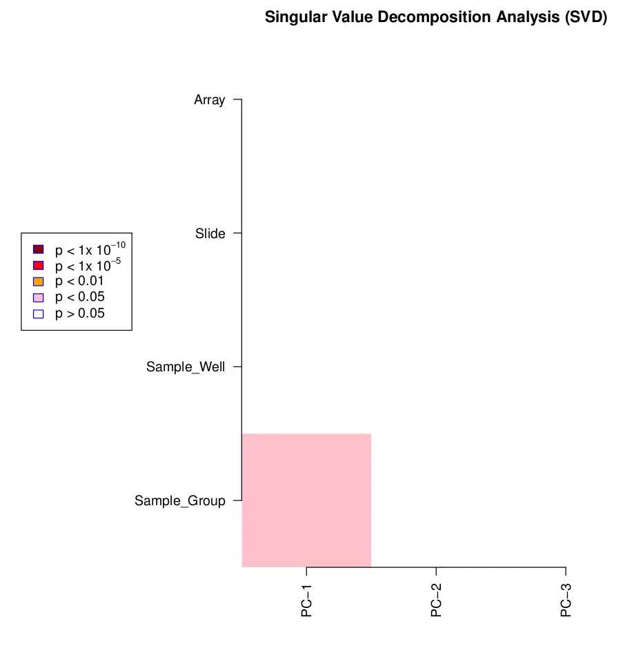
image.png

上图是用自带的测试数据绘制的，不是很复杂，看不出来。下图用 GSE40279 的 656 个样本绘制的。其中年龄是数字变量，其他都为分类变量。

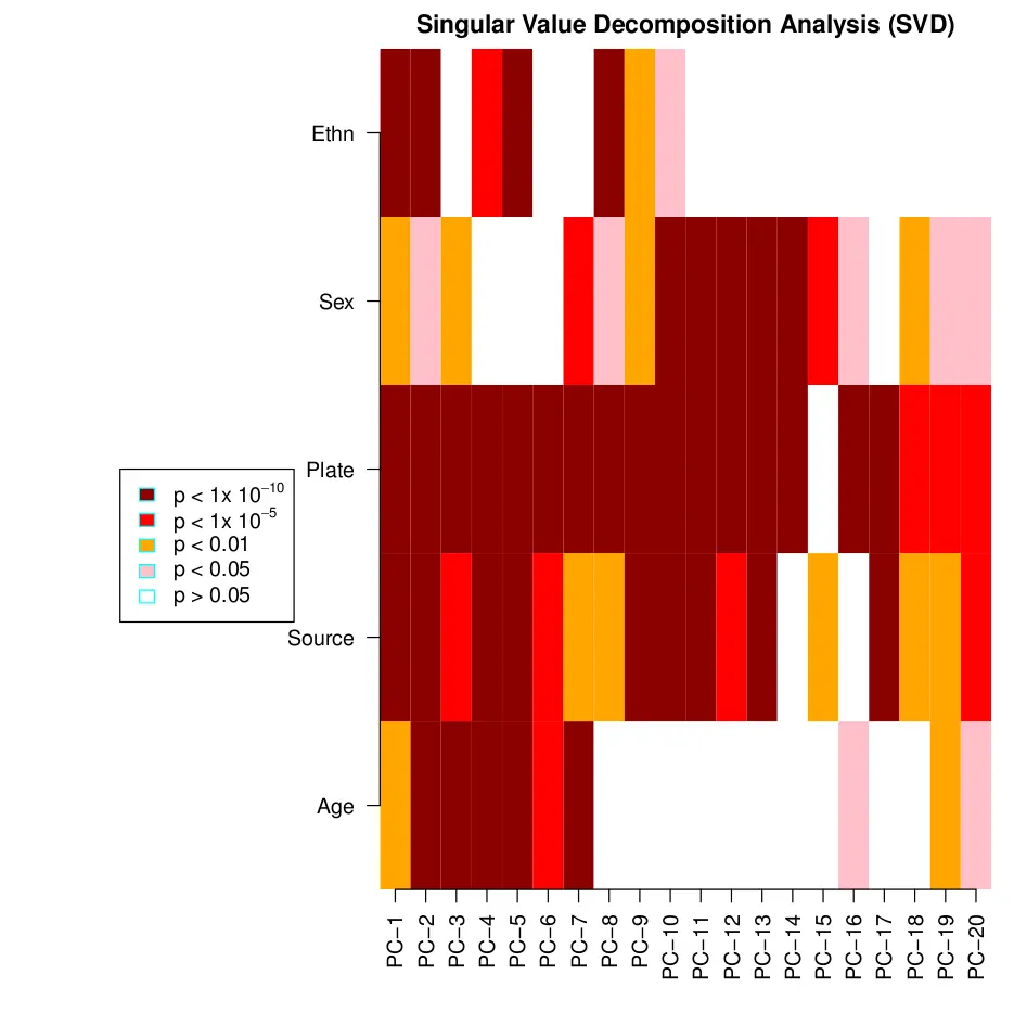
image.png

6.6 Batch Effect Correction

ComBat 方法是 sva 包里的一个方法，已经整合到 ChAMP 包里了，batchname=c(“Slide”) 参数控制矫正因素。champ.runCombat() 函数自动把 Sample_Group 作为协变量矫正，现在又加入了另一个参数 variablename 用来加入自己的协变量进行矫正。如果用户在 champ.runCombat() 函数中写的 batchname 正确，函数将自动进行批次效应矫正。
ComBat 如果直接用 beta 值进行矫正，输出可能不在 0-1 之间，所以计算机在计算前需要做一个变换。如果用 M-values 矫正，参数 logitTrans=FALSE 设置。有时候批次效应和变异会混杂在一起，如果矫正了批次效应，变异也会消失，

#矫正批次效应，这步非常耗时。
myCombat <- champ.runCombat(beta=myNorm,pd=myLoad$pd,batchname=c("Slide"))
#查看矫正后 的结果
champ.SVD()

6.7 Differential Methylation Probes（DMP & DMR & DMB)

目的是找出几百万 CpG 中的哪些在疾病中发生了变化，而这些变化又是如何导致了基因发生了变化，最终导致了人体生病。

DMP 代表找出 Differential Methylation Probe（差异化 CpG 位点），DMR 代表找出 Differential Methylation Region（差异化 CpG 区域），Block 代表 Differential Methylation Block（更大范围的差异化 region 区域）。

champ.DMP() 实现了 limma 包中利用 linear model 计算差异甲基化位点的 p-value。最新的 champ.DMP()包支持分析数值型变量如年龄，分类型变量如包含多个表型的：“tumor”, “metastasis”, “control”。数值型变量（如年龄）会用 linear regression 模型作为协变量进行分析，to find your covariate-related CpGs, say age-related CpGs. 分类型变量会按类型分类进行比较，如比较 “tumor–metastatic”, “tumor-control”, and “metastatis-control” 之间的差异，结果会输出一个数据框，包含差异的探针：P-value, t-statistic and difference in mean methylation（被转换为 logFC，类似于 RNA-seq 中的 log fold-change）。还包括每个探针的注释，相同组的平均 beta 值，两组之间的 delta beta 值（与 logFC 相同的意思，老版本的包需要）。高级用户可以用 limma 包进一步用输出的探针及 p 值进行 DMR 分析。

#DMPs 分析
myDMP <- champ.DMP(beta = myNorm,pheno=myLoad$pd$Sample_Group)
#查看结果
head(myDMP[[1]])

champ.DMP() 返回的是 list，新版本的 ChAMP 包含 GUI 交互界面检查 myDMP 的结果。用户提供未经修改的 champ.DMP (myDMP) 函数产生的 orginal beta matrix 结果和 covariates，DMP.GUI() 函数自动检测 covariates 是数值型还是分类型。分类型如 case/control， DMP.GUI() 自动画出显著性差异位点。

DMP.GUI(DMP=myDMP[[1]],beta=myNorm,pheno=myLoad$pd$Sample_Group)
# myDMP is a list now, each data frame is stored as myDMP[[1]], myDMP[[2]], myDMP[[3]]...

6.7.2 Hydroxymethylation Analysis 羟甲基化

一些用户想做羟甲基化，下面为示例代码

myDMP <- champ.DMP(beta=myNorm, pheno=myLoad$pd$Sample_Group, compare.group=c("oxBS", "BS"))
# In above code, you can set compare.group() as "oxBS" and "BS" to do DMP detection between hydroxymethylatio and normal methylation.
hmc <- myDMP[[1]][myDMP[[1]]$deltaBeta>0,]
# Then you can use above code to extract hydroxymethylation CpGs.

6.8 Differential Methylation Regions 差异甲基化区域

DMRs 主要指一连串的 CpG 都会出现很明显的差异，champ.DMR() 函数计算并返回一个数据框，包括：detected DMRs, with their length, clusters, number of CpGs annotated.
函数包含三种算法 Bumphunter, ProbeLasso and DMRcate. Bumphunter 比较可靠，精确度可以有 90% 以上，ProbeLasso 有 75% 左右，DMRcate 是后来集成进去的，没有评测过。Bumphunter 算法首先将所有的探针分成几小类，然后用随机 permutation 方法评估候选的 DMRs.

myDMR <- champ.DMR(beta=myNorm,pheno=myLoad$pd$Sample_Group,method="Bumphunter")
head(myDMR$DMRcateDMR)
DMR.GUI(DMR=myDMR)
# It might be a little bit slow to open DMR.GUI() because function need to extract annotation for CpGs from DMR. Might take 30 seconds.

6.9 Differential Methylation Blocks

在 Block-finder 功能中，champ.Block() 函数首先在全基因组范围上计算 small clusters (regions) ，然后对于每个 cluster，计算平均值和位置，将每个区域压缩为一个单元。 When we finding DMB, only single unit from open sea would be used to do clustering. Here Bumphunter algorithm will be used to find “DMRs” over these regions (single units after collapse). In our previous paper23, and other scientists’ work24 we demonstrated that Differential Methylated Blocks may show universal feature across various cancers

myBlock <- champ.Block(beta=myNorm,pheno=myLoad$pd$Sample_Group,arraytype="450K")
head(myBlock$Block)
Block.GUI(Block=myBlock,beta=myNorm,pheno=myLoad$pd$Sample_Group,runDMP=TRUE,compare.group=NULL,arraytype="450K")

6.10 Gene Set Enrichment Analysis

寻找作用通路网络中的疾病关联小网络
After previous steps, you may already get some significant DMPs or DMRs, thus you may want to know if genes involved in these significant DMPs or DMRs are enriched for specific biological terms or pathways. To achieve this analysis, you can use champ.GSEA() to do GSEA analysis.champ.GSEA() would automatically extract gene information, transfer CpG information into gene information then conduct GSEA on each list.

There are two ways to do GSEA. In previous version, ChAMP used pathway information downloaded from MSigDB. Then Fisher Exact Test will be used to calculate the enrichment status of each pathway. After gene enrichment analysis, champ.GSEA() function would automatically return pathways with P-value smaller then adjPval cutoff.

However, as pointed out by Geeleher [citation], since different genes has different numbers of CpGs contained inside, the two situation that one genes with 50 CpGs inside but only one of them show significant methylation, and one gene with 2 CpGs inside but two are significant methylated should not be eaqualy treated. The solution is use number of CpGs contained by genes to correct significant genes. as implemented in the gometh function from missMethyl package25. In gometh function, it used number of CpGs contained by each gene replace length as biased data, to correct this issue. The idea of gometh is fitting a curve for numbers of CpGs across genes related with GSEA, then using the probability weighting function to correct GO’s p value.

champ.GSEA() function as “goseq” to use goseq method to do GSEA, or user may set it as “fisher” to do normal Gene Set Enrichment Analysis.

myGSEA <- champ.GSEA(beta=myNorm,DMP=myDMP[[1]], DMR=myDMR, arraytype="450K",adjPval=0.05, method="fisher")
# myDMP and myDMR could (not must) be used directly.

6.11 Differential Methylated Interaction Hotspots

champ.EpiMod() This function uses FEM package to infer differentially methylated gene modules within a user-specific functional gene-network. This network could be e.g. a protein-protein interaction network. Thus, the champ.EpiMod() function can be viewed as a functional supervised algorithm, which uses a network of relations between genes (usually a PPI network), to identify subnetworks where a significant number of genes are associated with a phenotype of interest (POI). The EpiMod algorithm can be run in two different modes: at the probe level, in which case the most differentially methylated probe is assigned to each gene, or at the gene-level in which case a DNAm value is assigned to each gene using an optimized procedure described in detail in Jiao Y, Widschwendter M, Teschendorff AE Bioinformatics 2014. Originally, the FEM package was developed to infer differentially methylated gene modules which are also deregulated at the gene expression level, however here we only provide the EpiMod version, which only infers differentially methylated modules. More advanced user may refer to FEM package for more information.

myEpiMod <- champ.EpiMod(beta=myNorm,pheno=myLoad$pd$Sample_Group)

6.13 Cell Type Heterogeneity

由于 DNA 甲基化有高的细胞特异性，许多 DMPs/DMRs 的变化是由细胞成分导致的。许多方法可以矫正这个问题：RefbaseEWAS 用组织的细胞类型做参考数据库，确定细胞比例。In ChAMP, we include a reference databases for whole blood, one for 27K and the other for 450K. After champ.refbase() function, cell type heterogeneity corrected beta matrix, and cell-type specific proportions in each sample will be returned. Do remember champ.refbase() can only works on Blood Sample Data Set.

myRefBase <- champ.refbase(beta=myNorm,arraytype="450K")
# Our test data set is not whole blood. So it should not be run here.

阅读推荐：

生信技能树公益视频合辑：学习顺序是 linux，r，软件安装，geo，小技巧，ngs 组学！

B 站链接：https://m.bilibili.com/space/338686099

YouTube 链接：https://m.youtube.com/channel/UC67sImqK7V8tSWHMG8azIVA/playlists

生信工程师入门最佳指南：https://mp.weixin.qq.com/s/vaX4ttaLIa19MefD86WfUA

学徒培养：https://mp.weixin.qq.com/s/3jw3_PgZXYd7FomxEMxFmw

更多精彩内容，就在简书 APP

“谢谢您对知识的尊重！”

还没有人赞赏，支持一下

Richard_Zhou上海交大遗传学博士在读，生物信息学 / 机器学习 / Python/R / 爱好者
邮件 weisjt…

总资产 9 共写了 2.6W 字获得 182 个赞共 349 个粉丝

被以下专题收入，发现更多相似内容

推荐阅读更多精彩内容

• 电脑配置情况 操作系统：Win10 使用原则 别把电脑当成硬盘存东西 SSD 用来快速运行的，用来存储的 尽量不使用…
  
  俊学之道阅读 218 评论 0 赞 1
• 最近在弄一个 iOS 的嵌入统一的功能，大费脑细胞…… 各种坑，网上找了很多帖子方法，虽然我比较懒，很少整理发表…
  
  
• 我生活在一个四周封闭的山沟沟里，没什么眼界，不是看到山就是看到水的，日子简单明了，在哪里我只需要做点简单的事，做个…
  
  融化的心阅读 235 评论 0 赞 0
• 在以前的单位，微信运动只有 5、6 千。来了总部，随随便便上万步，注意这个数据统计只是我在总部大楼里的步数哦。每日穿梭…
  https://www.jianshu.com/p/7993b890e4f3