OpenCV 系列教程 5 | OpenCV 图像处理（中）

霍夫变换

基本概念

霍夫变换是一种特征提取技术，主要应用于检测图像中的直线或者圆。
OpenCV 中分为霍夫线变换和霍夫圆变换。

霍夫线变换

分类

• 标准霍夫变换（SHT） cv2.HoughLines
• 多尺度霍夫变换 （MSHT） cv2.HoughLines
• 累计概率霍夫变换 （PPHT） cv2.HoughLinesP

注意：在使用霍夫线变换之前，首先要对图像进行边缘检测的处理，即霍夫线变换的直接输入只能是边缘二值图像

标准霍夫变换

使用极坐标来表示直线，对于在笛卡尔坐标上直线上所有给定的点，在极坐标上都能转换成正弦曲线，直线上所有点绘制出来的正弦曲线交与一点，若交于交点的曲线数量超过一定阈值，说明在笛卡尔坐标上表示一条直线。更多资料

HoughLines(image, rho, theta, threshold[, lines[, srn[, stn[, min_theta[, max_theta]]]]]) -> lines

• image: 输入图像，需为 8 位的单通道二进制图像
• rho: 以像素为单位的距离精度
• theta: 以弧度为单位的角度精度
• threshold: 阈值参数
• srn: 默认值为 0 对于多尺度霍夫变换，srn 表示进步尺寸 rho 的除数距离，粗略的累加器进步尺寸直接是 rho ，而精确的累加器进步尺寸为 rho/srn。
• stn: 默认值为 0 对于多尺度霍夫变换，stn 表示进步尺寸的单位角度 theta 的除数距离。若 srn stn 同时为 0，表示使用经典的霍夫变换，否则这两个参数都应该是正数。

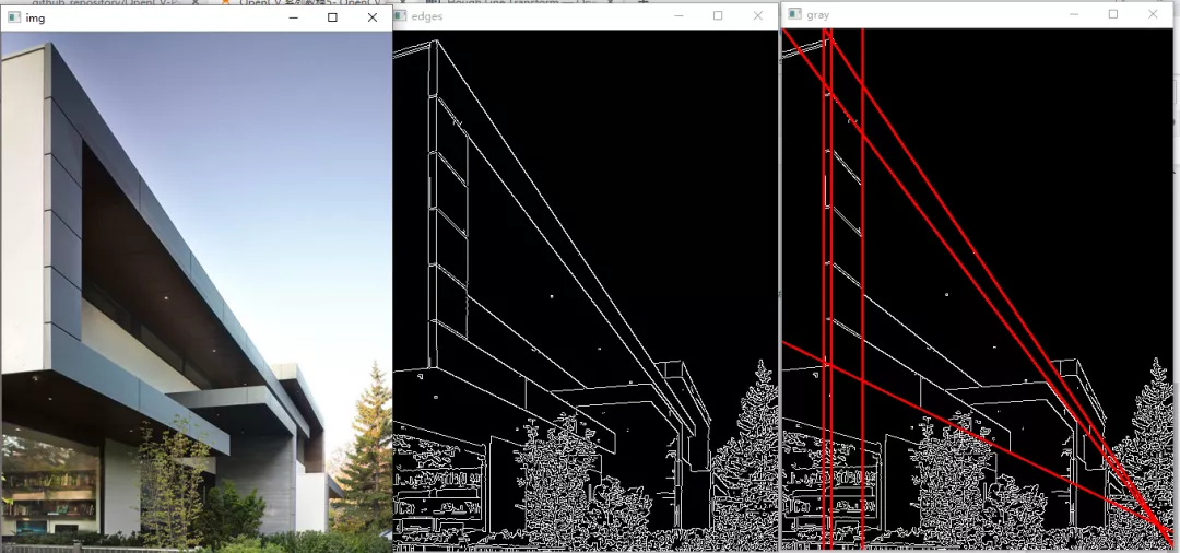
import cv2
import numpy as np
img = cv2.imread("./sample_img/HoughLines.jpg")
edges = cv2.Canny(img, 50, 200, apertureSize=3)
gray = cv2.cvtColor(edges, cv2.COLOR_GRAY2BGR)
# 经典的霍夫变换
lines = cv2.HoughLines(edges, 1, np.pi/180, 180, 0, 0) # 在图像中找到的所有直线都存储在这里
for i in range(lines.shape[0]-1):
    rho, theta = lines[i][0][0], lines[i][0][1] # rho 为距离， theta 为角度，把每条直线的参数分离出来
    # 坐标转换
    a = np.cos(theta)
    b = np.sin(theta)
    x0 = a*rho
    y0 = b*rho
    x1 = int(x0 + 1000*(-b))
    y1 = int(y0 + 1000*(a))
    x2 = int(x0 - 1000*(-b))
    y2 = int(y0 - 1000*(a))
    # 绘制直线
    cv2.line(gray, (x1, y1), (x2, y2), (0, 0, 255), 2)
cv2.imshow("img", img)    
cv2.imshow("gray", gray)
cv2.imshow("edges", edges)
cv2.waitKey(0)
cv2.destroyAllWindows()

图像卷积与滤波的一些知识点)

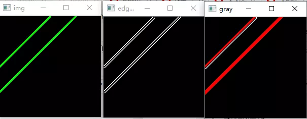
注意，下面的坐标变换不是很清楚

img = np.zeros((200, 200, 3), dtype=np.uint8)
cv2.line(img, (0, 100), (100, 0), (0, 255, 0), 2)
cv2.line(img, (0, 150), (150, 0), (0, 255, 0), 2)
edges = cv2.Canny(img, 50, 200, apertureSize=3)
gray = cv2.cvtColor(edges, cv2.COLOR_GRAY2BGR)
# 经典的霍夫变换
lines = cv2.HoughLines(edges, 1, np.pi/180, 100, 0, 0) # 在图像中找到的所有直线都存储在这里
for i in range(lines.shape[0]-1):
    rho, theta = lines[i][0][0], lines[i][0][1] # rho 为距离， theta 为角度，把每条直线的参数分离出来
    # 坐标转换
    a = np.cos(theta)
    b = np.sin(theta)
    x0 = a*rho
    y0 = b*rho
    x1 = int(x0 + 1000*(-b))
    y1 = int(y0 + 1000*(a))
    x2 = int(x0 - 1000*(-b))
    y2 = int(y0 - 1000*(a))
    # 绘制直线
    cv2.line(gray, (x1, y1), (x2, y2), (0, 0, 255), 2)
cv2.imshow("img", img)    
cv2.imshow("gray", gray)
cv2.imshow("edges", edges)
cv2.waitKey(0)
cv2.destroyAllWindows()

累计概率霍夫变换

累计概率霍夫变换可以找出图像中直线大概的起始和终止坐标，返回 4 个元素，分别代表起始坐标（x1, y1）,终止坐标（x2, y2）

HoughLinesP(image, rho, theta, threshold[, lines[, minLineLength[, maxLineGap]]]) -> lines

• image: 输入图像，需为 8 位单通道二进制图像
• rho: 以像素为单位的距离精度，另一种表述方式是：直线搜索时的进步尺寸的单位半径
• theta: 以弧度为单位的角度精度，另一种表述方式是：直线搜索时的进步尺寸的单位角度
• threshold: 阈值参数
• lines: 存储检测到的线条的输出矢量，返回 4 个元素，分别代表起始坐标（x1, y1）,终止坐标（x2, y2）
• minLineLength: 默认值 0 表示最低线段的长度，比这个设定参数短的线段不能显示出来
• maxLineGap: 默认值 0 允许将同一行点与点之间连接起来的最大的距离。

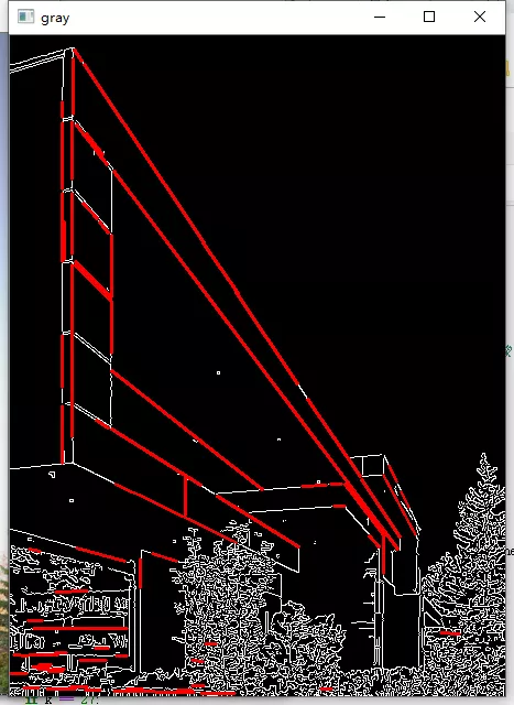
import cv2
import numpy as np
img = cv2.imread("./sample_img/HoughLines.jpg")
edges = cv2.Canny(img, 50, 200, apertureSize=3) # 边缘检测出来就是二值图像
gray = cv2.cvtColor(edges, cv2.COLOR_GRAY2BGR)
threshold = 80
minLineLength = 40
maxLineGap = 10
linesP = cv2.HoughLinesP(edges, 1, np.pi/180, threshold, minLineLength, maxLineGap)
for i in range(linesP.shape[0]):
    x1 = linesP[i][0][0]
    y1 = linesP[i][0][1]
    x2 = linesP[i][0][2]
    y2 = linesP[i][0][3]
    cv2.line(gray, (x1, y1), (x2, y2), (0, 0, 255), 2)
cv2.imshow("img", img)    
cv2.imshow("gray", gray)
cv2.imshow("edges", edges)
cv2.waitKey(0)
cv2.destroyAllWindows()

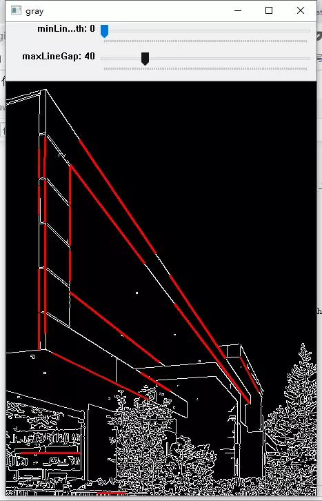
import cv2
import numpy as np
def nothing(x):
    pass
img = cv2.imread("./sample_img/HoughLines.jpg")
edges = cv2.Canny(img, 50, 200, apertureSize=3) # 边缘检测出来就是二值图像
cv2.namedWindow("gray")
cv2.createTrackbar("minLineLength", "gray", 0, 200, nothing)
cv2.createTrackbar("maxLineGap", "gray", 0, 200, nothing)
while(1):
    gray = cv2.cvtColor(edges, cv2.COLOR_GRAY2BGR)
    minLineLength = cv2.getTrackbarPos("minLineLength", "gray")
    maxLineGap = cv2.getTrackbarPos("maxLineGap", "gray")
    linesP = cv2.HoughLinesP(edges, 1, np.pi/180, 70, minLineLength, maxLineGap)
    for i in range(linesP.shape[0]):
        x1 = linesP[i][0][0]
        y1 = linesP[i][0][1]
        x2 = linesP[i][0][2]
        y2 = linesP[i][0][3]
        cv2.line(gray, (x1, y1), (x2, y2), (0, 0, 255), 2)
    k = cv2.waitKey(1) & 0xff
    if k == 27:
        break
    #cv2.imshow("img", img)    
    cv2.imshow("gray", gray)
    #cv2.imshow("edges", edges)
cv2.destroyAllWindows()

霍夫圆变换

原理

圆的表达式为 $(x-a)^{2} + (y-b)^{2} = r^{2}$ ，将圆上的任意点 (x, y) 变换成 (a, b, r) 坐标结果是一个圆锥，同一个圆上的点形成的圆锥会交于一点，从该交点可以得出圆的信息。

HoughCircles(image, method, dp, minDist[, circles[, param1[, param2[, minRadius[, maxRadius]]]]]) -> circles

• image:输入图像，需为 8 位单通道二进制图像
• method: 使用的检测方法，目前只有 cv2.HOUGH_GRADIENT 霍夫梯度法一种
• dp: 用来检测圆心的累加器图像的分辨率于输入图像之比的倒数，且此参数允许创建一个比输入图像分辨率低的累加器。例如，如果dp= 1时，累加器和输入图像具有相同的分辨率。如果dp=2，累加器便有输入图像一半那么大的宽度和高度。
• minDist: 为霍夫变换检测到的圆的圆心之间的最小距离，即让我们的算法能明显区分的两个不同圆之间的最小距离。这个参数如果太小的话，多个相邻的圆可能被错误地检测成了一个重合的圆。反之，这个参数设置太大的话，某些圆就不能被检测出来了。
• param1: 有默认值100。它是参数method设置的检测方法的对应的参数。对当前唯一的方法霍夫梯度法CV_HOUGH_GRADIENT，它表示传递给canny边缘检测算子的高阈值，而低阈值为高阈值的一半。
• param2: 有默认值100。它是参数method设置的检测方法的对应的参数。对当前唯一的方法霍夫梯度法CV_HOUGH_GRADIENT，它表示在检测阶段圆心的累加器阈值。它越小的话，就可以检测到更多根本不存在的圆，而它越大的话，能通过检测的圆就更加接近完美的圆形了。
• minRadius: int类型的minRadius,有默认值0，表示圆半径的最小值。
• maxRadius: int类型的maxRadius,也有默认值0，表示圆半径的最大值。
• circles: 返回的结果，包含三个元素 (x, y, radius)，圆心和半径

图片例程

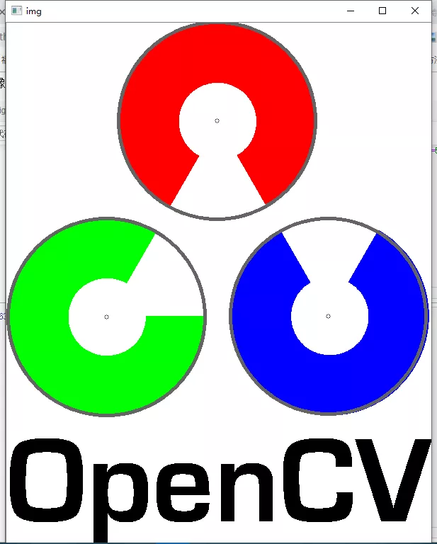
import cv2
import numpy as np
"""
img = np.zeros((200, 200, 3), dtype=np.uint8)
cv2.circle(img, (100, 100), 50, (0, 255, 255))
cv2.circle(img, (95, 100), 50, (0, 255, 255))
cv2.circle(img, (80, 100), 50, (0, 255, 255))
"""
img = cv2.imread("./sample_img/opencv-logo.png")
img1 = cv2.imread("./sample_img/opencv-logo.png", 0)
gray = cv2.cvtColor(img, cv2.COLOR_BGR2GRAY)
gaussian = cv2.GaussianBlur(gray, (9, 9), 2, 2)
circle = cv2.HoughCircles(gaussian, cv2.HOUGH_GRADIENT, dp=1, minDist=20, param1=50, param2=50, minRadius=0, maxRadius=0)
for i in range(circle.shape[1]):
    center = (circle[0][i][0], circle[0][i][1])
    radius = circle[0][i][2]
    cv2.circle(img, center, radius, (100, 100, 100), 4)
    cv2.circle(img, center, 3, (100, 100, 100))
cv2.imshow("img", img)
cv2.imshow("img1", cv2.Canny(img1, 50, 200, apertureSize=3))
cv2.imshow("gray", gray)
cv2.waitKey(0)
cv2.destroyAllWindows()

视频例程

import cv2
cap = cv2.VideoCapture(0)
# 设置摄像头分辨率
cap.set(cv2.CAP_PROP_FRAME_WIDTH, 400)
cap.set(cv2.CAP_PROP_FRAME_HEIGHT, 400)
while(1):
    # 提取每一帧, frame 源视频
    _, frame = cap.read()
    frame = cv2.flip(frame, 1)
    gray = cv2.cvtColor(frame, cv2.COLOR_BGR2GRAY)
    #gaussian = cv2.GaussianBlur(gray, (9, 9), 2, 2)
    #canny = cv2.Canny(gaussian, 20, 100)
    circle = cv2.HoughCircles(gray, cv2.HOUGH_GRADIENT, dp=1,
                              minDist=20, param1=50, param2=50, minRadius=0, maxRadius=0)
    if circle is not None:
        center = (circle[0][0][0], circle[0][0][1])
        radius = circle[0][0][2]
        cv2.circle(frame, center, radius, (0, 0, 255), 4)
    cv2.imshow("frame", frame)  # 源视频
    #cv2.imshow("gray", gray) # 源视频
    k = cv2.waitKey(1) & 0xFF
    if k == 27:
        break
cap.release()  # 记得释放掉捕获的视频
cv2.destroyAllWindows()

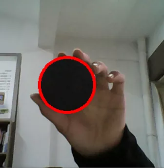
效果并不是很好，是由于霍夫变换存在一定缺陷

更多资料

霍夫圆变换原理)

重映射

基本概念

重映射：把一副图像中某位置的像素放置到另一个图片指定位置的过程，为了完成映射过程，需要获得一些插值为非整数像素的坐标，因为原图像和目标图像的像素坐标是不一一对应的。

remap(src, map1, map2, interpolation[, dst[, borderMode[, borderValue]]]) -> dst

• src: 源图像
• map1: 1.表示点 (x, y) 的第一个映射 2.表示 CV_16SC2、CV_32FC1、或 CV_32FC2 类型的 X 值
• map2: 根据 map1 参数来确定表示的对象，1. 若 map1 表示点 (x, y) 时，该参数不代表任何值 2. 表示 CV_16UC1、CV_32FC1 类型的 Y 值
• interpolation: 插值的参数，在原图找不到的坐标使用插值补全
• borderMode: 边界模式
• borderValue:

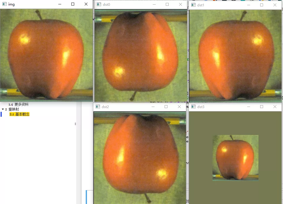
例程

import cv2
def remap_mode(mode, map_x, map_y):
    if mode == 0:   # 倒置
        for i in range(map_x.shape[0]):
            map_x[i,:] = [x for x in range(map_x.shape[1])]
        for j in range(map_y.shape[1]):
            #map_y[:,j] = [map_y.shape[0]-y for y in range(map_y.shape[0])]  
            map_y[:,j] = [map_y.shape[0]-y-1 for y in range(map_y.shape[0])]  
    elif mode == 1: # 竖直对称
        for i in range(map_x.shape[0]):
            map_x[i,:] = [map_x.shape[1]-x for x in range(map_x.shape[1])]
        for j in range(map_y.shape[1]):
            map_y[:,j] = [y for y in range(map_y.shape[0])]        
    elif mode == 2: # mode=0 和 mode=1 的组合
        for i in range(map_x.shape[0]):
            map_x[i,:] = [map_x.shape[1]-x for x in range(map_x.shape[1])]
        for j in range(map_y.shape[1]):
            map_y[:,j] = [map_y.shape[0]-y for y in range(map_y.shape[0])]
    elif mode == 3: # 缩小后在中间显示
        for i in range(map_x.shape[0]):
            for j in range(map_x.shape[1]):
                if j > map_x.shape[1]*0.25 and j < map_x.shape[1]*0.75 and i > map_x.shape[0]*0.25 and i < map_x.shape[0]*0.75:
                    map_x[i,j] = 2 * (j-map_x.shape[1]*0.25) + 0.5
                    map_y[i,j] = 2 * (i-map_y.shape[0]*0.25) + 0.5
                else:
                    map_x[i,j] = 0
                    map_y[i,j] = 0
#img = cv2.imread("./sample_img/apple.jpg")
img = cv2.imread("./sample_img/Back_Projection_Theory2.jpg", 0)
# 创建两个映射矩阵 x, y 
map_x = np.zeros((img.shape[0], img.shape[1]), dtype=np.float32)
map_y = np.zeros((img.shape[0], img.shape[1]), dtype=np.float32)
cv2.imshow("img", img)
for i in range(4):
    remap_mode(i, map_x, map_y)
    dst = cv2.remap(img, map_x, map_y, cv2.INTER_LINEAR)    
    cv2.imshow("dst"+str(i), dst)
    #print(map_x, map_y, map_x.shape, map_y.shape)
cv2.waitKey(0)
cv2.destroyAllWindows()

部分参数解释（以倒置为例）

img = np.array(np.arange(10, 30).reshape(4, 5), dtype=np.uint8)
map1 = np.zeros((img.shape[0], img.shape[1]), dtype=np.float32)
map2 = np.zeros((img.shape[0], img.shape[1]), dtype=np.float32)
# 倒置
for i in range(map1.shape[0]):
    map1[i,:] = [x for x in range(map1.shape[1])] # 行坐标
for j in range(map2.shape[1]):
    map2[:,j] = [map2.shape[0]-y-1 for y in range(map2.shape[0])]  # 列坐标
print(map1, map2, sep='\n')    
print(img, cv2.remap(img, map1, map2, cv2.INTER_LINEAR), sep='\n')

[[0. 1. 2. 3. 4.]
 [0. 1. 2. 3. 4.]
 [0. 1. 2. 3. 4.]
 [0. 1. 2. 3. 4.]]
[[3. 3. 3. 3. 3.]
 [2. 2. 2. 2. 2.]
 [1. 1. 1. 1. 1.]
 [0. 0. 0. 0. 0.]]
[[10 11 12 13 14]
 [15 16 17 18 19]
 [20 21 22 23 24]
 [25 26 27 28 29]]
[[25 26 27 28 29]
 [20 21 22 23 24]
 [15 16 17 18 19]
 [10 11 12 13 14]]

cv2.remap() 函数中的 map1, map2 参数代表目标图中的 (x,y) 点在原图中的 x 坐标（由map2提供）与 y 坐标（由map1提供）待定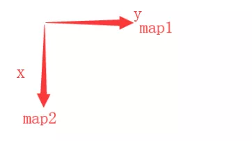

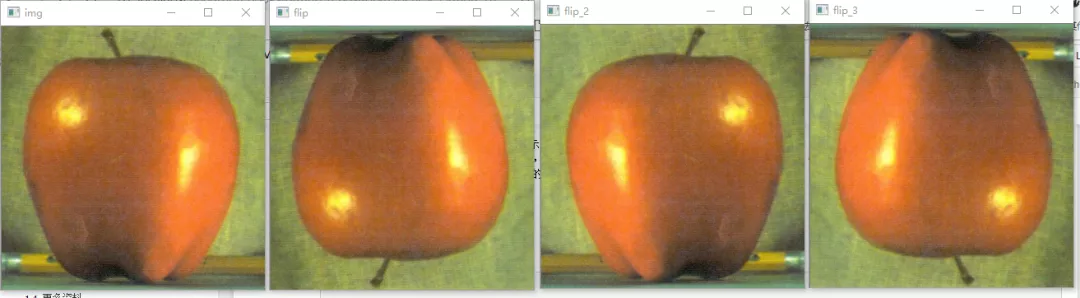
与 cv2.flip() 函数比较

flip(src, flipCode[, dst]) -> dst

• src: 源图像
• flipCode: 变换代码
  • 0: 倒影
  • 1: 左右镜面
  • 2: 0+1 的效果

import cv2
img = cv2.imread("./sample_img/apple.jpg")
flip = cv2.flip(img, 0)
flip_2 = cv2.flip(img, 1)
flip_3 = cv2.flip(img, -1)
cv2.imshow("img", img)
cv2.imshow("flip", flip)
cv2.imshow("flip_2", flip_2)
cv2.imshow("flip_3", flip_3)
cv2.waitKey(0)
cv2.destroyAllWindows()

直方图

直方图基本概念，分析

学习目标：

• OpenCV 和 Numpy 中的函数查找直方图
• 绘制直方图
• cv2.calcHist(), np.histogram(), plt.hist()

直方图就是灰色图像每个像素，横坐标代表像素值（0 - 255），纵坐标代表每个像素值的个数。直方图可以直观了解该图像的对比度，亮度，强度分布。
类似：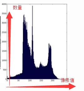

OpenCV 中的直方图计算函数

calcHist(images, channels, mask, histSize, ranges[, hist[, accumulate]]) -> hist

• images: uint8 或者 float32 类型的图像， 使用时格式为 [img]
• channels: 通道标识，若图像为灰度图，则使用 [0]，彩色图用 [0], [1], [2] 分别代表蓝绿红通道的直方图
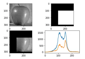
• mask: 掩模，抽取图像中的某块区域时使用，创建的掩模白底就是目标区域，否则为黑色，mask 大小需与原图一致
• histSize: 量程，代表直方图横坐标的最大值，对于图像来说使用 [256]
• range: 像素值的范围 [0, 256]
• hist: 返回一个序列，代表每个像素值的数量

import cv2
import numpy as np
img = cv2.imread("./sample_img/apple.jpg")
hsv = cv2.cvtColor(img, cv2.COLOR_BGR2HSV)
hue = np.zeros(hsv.shape, dtype=np.uint8)
hue = cv2.mixChannels(hsv, hue, [0, 0])
hist = cv2.calcHist(hue, [0], None, [180], [0, 180]) # 返回的是 (0, 256) 每个像素值的个数

Numpy 中的直方图计算函数

import numpy as np
hist, bins = np.histogram(img.ravel(), 256, [0, 256])

hist = np.bincount(img.ravel(), minlength=256)

对于一维直方图，使用 np.bincount() 的速度比 np.histogram() 快 10 倍，但是 OpenCV 的方法更快，所以还是使用 OpenCV 的直方图方法

直方图的绘制

plt.hist(x, bins=None, range=None, density=None, weights=None, cumulative=False, bottom=None, histtype='bar', align='mid', orientation='vertical', rwidth=None, log=False, color=None, label=None, stacked=False, normed=None, *, data=None, **kwargs)

• x: 序列或者数组，大小为 (n, )
• bins: 在直方图中（像素值），代表将 256 等分的分数
• range: 像素值的范围，例如 (0, 256)

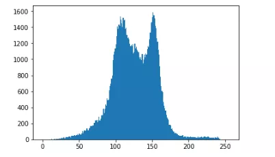
import cv2
import matplotlib.pyplot as plt
img = cv2.imread("./sample_img/apple.jpg", 0)
plt.hist(img.ravel(), 256, [0, 256])
plt.show()

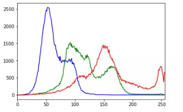
import cv2
import numpy as np
import matplotlib.pyplot as plt
img = cv2.imread('./sample_img/apple.jpg')
color = ('b', 'g', 'r')
for i, col in enumerate(color):
    histr = cv2.calcHist([img], [i], None, [256], [0, 256])
    plt.plot(histr, color=col)
    plt.xlim([0, 256]) # 横坐标限制在 0 - 256
plt.show()
cv2.imshow("img", img)

添加掩模

import cv2
import matplotlib.pyplot as plt
import numpy as np
img = cv2.imread('./sample_img/apple.jpg', 0)
# create a mask
mask = np.zeros(img.shape[:2], np.uint8)
mask[100:300, 100:400] = 255
masked_img = cv2.bitwise_and(img, img, mask=mask)
# Calculate histogram with mask and without mask
# Check third argument for mask
hist_full = cv2.calcHist([img], [0], None, [256], [0, 256])
hist_mask = cv2.calcHist([img], [0], mask, [256], [0, 256])
plt.subplot(221), plt.imshow(img, 'gray')
plt.subplot(222), plt.imshow(mask, 'gray')
plt.subplot(223), plt.imshow(masked_img, 'gray')
plt.subplot(224), plt.plot(hist_full), plt.plot(hist_mask)
plt.xlim([0, 256])
plt.show()

直方图均衡化

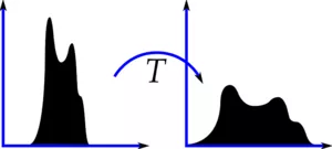
直方图均衡化被用来改善图像的对比度

直方图均衡化简单来说，就是把原始图像的直方图的分布均匀到所有像素。

均衡化

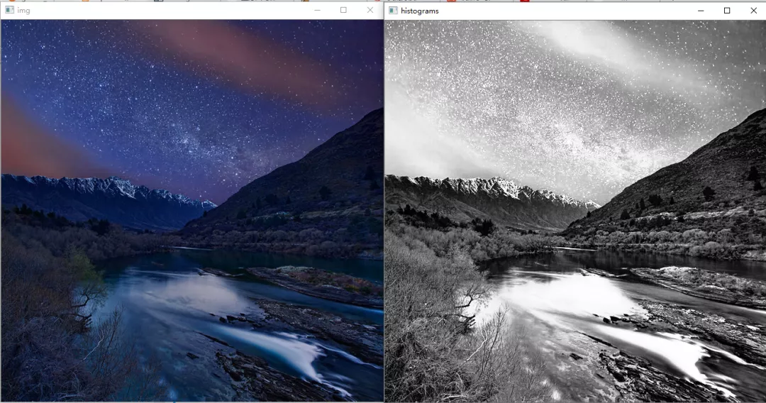
import cv2
img = cv2.imread("./sample_img/Histograms.jpg")
gray = cv2.cvtColor(img, cv2.COLOR_BGR2GRAY)
histograms = cv2.equalizeHist(gray)
cv2.imshow("img", img)
cv2.imshow("histograms", histograms)
cv2.waitKey(0)
cv2.destroyAllWindows()

对图像的灰度图像进行直方图均衡化

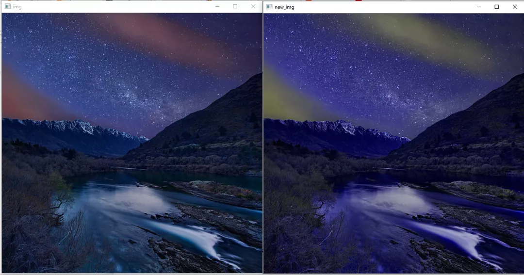
import cv2
img = cv2.imread("./sample_img/Histograms.jpg")
blue, green, red = cv2.split(img)
blue_histograms = cv2.equalizeHist(blue)
green_histograms = cv2.equalizeHist(green)
red_histograms = cv2.equalizeHist(red)
new_img = cv2.merge((blue_histograms, green_histograms, red_histograms))
cv2.imshow("img", img)
cv2.imshow("new_img", new_img)
cv2.waitKey(0)
cv2.destroyAllWindows()

对图像是 BGR 三通道进行直方图均衡化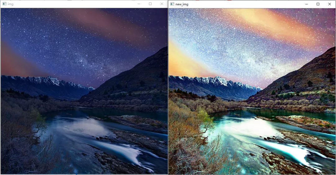

import cv2
img = cv2.imread("./sample_img/Histograms.jpg")
hsv = cv2.cvtColor(img, cv2.COLOR_BGR2HLS)
h, l, s = cv2.split(img)
#h = cv2.equalizeHist(h)
l = cv2.equalizeHist(l)
#s = cv2.equalizeHist(s)
new_img = cv2.merge((h, s, v))
cv2.imshow("img", img)
cv2.imshow("new_img", new_img)
cv2.waitKey(0)
cv2.destroyAllWindows()

对图像的 HLS 三通道的 L（亮度） 通道进行直方图均衡化

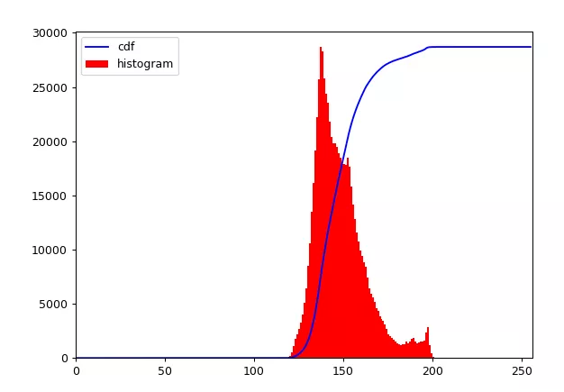
import cv2
import numpy as np
import matplotlib.pyplot as plt
img = cv2.imread('./sample_img/wiki.jpg', 0)
hist, bins = np.histogram(img.flatten(), 256, [0, 256])
cdf = hist.cumsum() # 返回一个给定轴上的元素的累积和
cdf_normalized = cdf * hist.max() / cdf.max()
plt.plot(cdf_normalized, color='b')
plt.hist(img.flatten(), 256, [0, 256], color='r')
plt.xlim([0, 256])
plt.legend(('cdf', 'histogram'), loc='upper left')
plt.show()

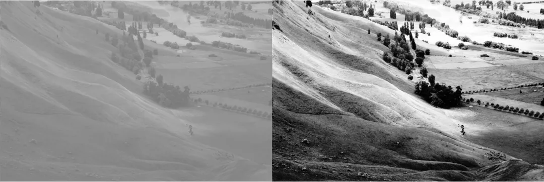
import cv2
import numpy as np
import matplotlib.pyplot as plt
img = cv2.imread('./sample_img/wiki.jpg', 0)
equ = cv2.equalizeHist(img)
new_img = np.hstack((img, equ))
cv2.imshow("new_img", new_img)
#cv2.imwrite("./sample_img/equalizeHist.jpg", new_img)
cv2.waitKey(0)
cv2.destroyAllWindows()

CLAHE (Contrast Limited Adaptive Histogram Equalization) 自适应均衡化

以上图像的均衡化使用的是全局的对比度，但有时候全局的对比度不一定是最好的，故引申出自适应均衡化

import numpy as np
import cv2
img = cv2.imread('./sample_img/tsukuba_l.png',0)
histograms = cv2.equalizeHist(img)
hstack_img = np.hstack((img, histograms))
cv2.imshow("hstack_img", hstack_img)
cv2.waitKey(0)
cv2.destroyAllWindows()

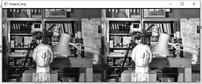
直方图均衡后背景对比度有所提高。但比较两个图像中的雕像的脸。由于亮度过高，我们丢失了大部分信息。这是因为它的直方图并不局限于特定区域。

自适应均衡化的原理是：图像被分成称为“tile”的小块（在OpenCV中，tileSize 默认为 8x8）。然后像往常一样对这些块中的每一个进行直方图均衡。所以在一个小区域内，直方图会限制在一个小区域（除非有噪音）。如果有噪音，它会被放大。为避免这种情况，应用对比度限制。如果任何直方图区间高于指定的对比度限制（在 OpenCV 中默认为 40 ），则在应用直方图均衡之前，将这些像素剪切并均匀分布到其他区间。均衡后，为了去除图块边框中的瑕疵，应用双线性插值。

cv2.createCLAHE([, clipLimit[, tileGridSize]]) -> retval

• clipLimit: 用于对比度限制的阈值
• tileGridSize: 用于直方图均衡化的网格大小。输入图像将被分割成大小相等的矩形块。tileGridSize 定义行和列中的块的数量。

apply(src, [, dst]) -> dst :利用对比度有限的自适应直方图均衡化来均衡灰度图像的直方图。

• src: CV_8UC1 类型的图像
• dst: 输出的图像

import numpy as np
import cv2
img = cv2.imread('./sample_img/tsukuba_l.png', 0)
# create a CLAHE object (Arguments are optional).
clahe = cv2.createCLAHE(clipLimit=2.0, tileGridSize=(8, 8))
cl1 = clahe.apply(img)
cv2.imshow('clahe_2', cl1)
cv2.waitKey(0)
cv2.destroyAllWindows()

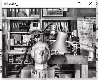
雕像区域的轮廓变得清晰可见了

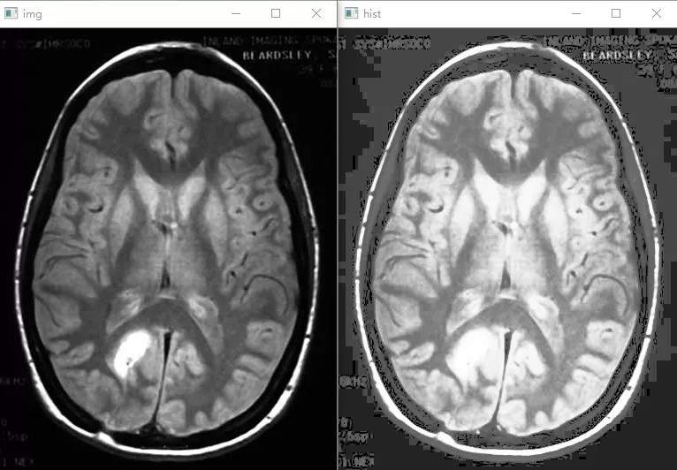
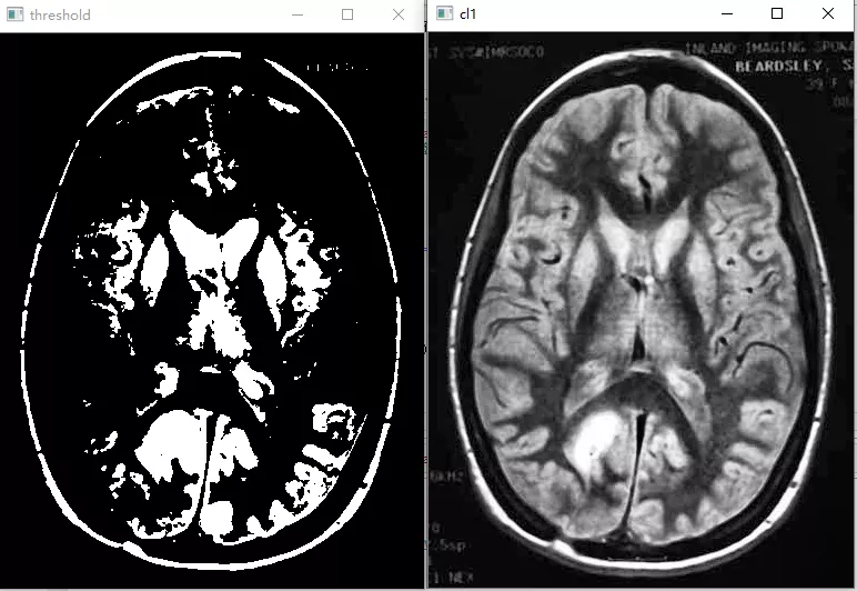
如何调整图像的对比度（附加的）

import cv2
import numpy as np
img = cv2.imread("./sample_img/brain.jpg", 0)
hist = cv2.equalizeHist(img)  # 直方图均衡
threshold = img.copy()
threshold[threshold > 127] = 255
threshold[threshold <= 127] = 0
clahe = cv2.createCLAHE(clipLimit=2.0, tileGridSize=(8, 8))
cl1 = clahe.apply(img)
cv2.imshow("img", img)
cv2.imshow("hist", hist)
cv2.imshow("threshold", threshold)
cv2.imshow("cl1", cl1)
cv2.waitKey(0)
cv2.destroyAllWindows()

2D 直方图

以上绘制的是一维直方图（只考虑一个特征，即灰度强度值），本节将讨论 2D 直方图，考虑两个特征（色调和饱和度），用于查找颜色直方图。

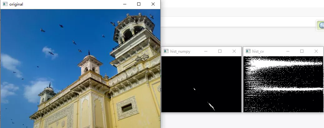
import cv2
import numpy as np
import matplotlib.pyplot as plt
img = cv2.imread("./sample_img/home.jpg")
hsv = cv2.cvtColor(img, cv2.COLOR_BGR2HSV)
# OpenCV 方法
# [0, 1] 代表 H 和 S 平面
# [190, 256] 180 是 H 平面最大幅值，256 是 S 平面最大幅值
hist_cv = cv2.calcHist([hsv], [0, 1], None, [180, 256], [0, 180, 0, 256])
# Numpy 方法
hist_numpy, xbins, ybins = np.histogram2d(hsv[0].ravel(), hsv[1].ravel(),
                                    [180, 256], [[0, 180], [0, 256]])
cv2.imshow("original", img)
cv2.imshow("hist_cv", hist_cv)
cv2.imshow("hist_numpy", hist_numpy)
cv2.waitKey(0)
cv2.destroyAllWindows()

plt.imshow(hist_cv, interpolation="nearest")

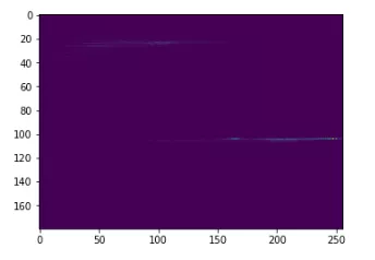
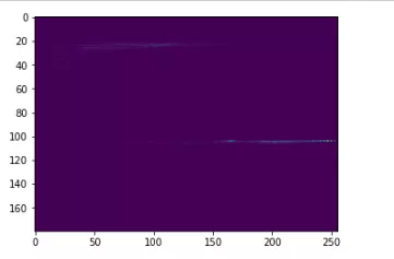
plt.imshow(hist_numpy, interpolation="nearest")

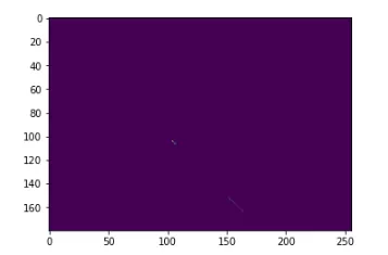
import cv2
import numpy as np
from matplotlib import pyplot as plt
img = cv2.imread('./sample_img/home.jpg')
hsv = cv2.cvtColor(img, cv2.COLOR_BGR2HSV)
hist = cv2.calcHist([hsv], [0, 1], None, [180, 256], [0, 180, 0, 256])
plt.imshow(hist, interpolation='nearest')
plt.show()

直方图比较

import cv2
base_img = cv2.imread("./sample_img/comparehist (1).jpg")
half_base = base_img[0:base_img.shape[0]//2, 0:base_img.shape[1]//2]
test_img = cv2.imread("./sample_img/comparehist (2).jpg")
test2_img = cv2.imread("./sample_img/comparehist (3).jpg")
base_hsv = cv2.cvtColor(base_img, cv2.COLOR_BGR2HSV)
half_hsv = cv2.cvtColor(half_base, cv2.COLOR_BGR2HSV)
test_hsv = cv2.cvtColor(test_img, cv2.COLOR_BGR2HSV)
test2_hsv = cv2.cvtColor(test2_img, cv2.COLOR_BGR2HSV)
base_hist = cv2.calcHist([base_hsv], [0, 1], None, [
                         180, 256], [0, 180, 0, 256])
half_hist = cv2.calcHist([half_hsv], [0, 1], None, [
                         180, 256], [0, 180, 0, 256])
test_hist = cv2.calcHist([test_hsv], [0, 1], None, [
                         180, 256], [0, 180, 0, 256])
test2_hist = cv2.calcHist([test2_hsv], [0, 1], None, [
                          180, 256], [0, 180, 0, 256])
base_hist = cv2.normalize(base_hist, base_hist, 0, 1, cv2.NORM_MINMAX, -1)
half_hist = cv2.normalize(half_hist, half_hist, 0, 1, cv2.NORM_MINMAX, -1)
test_hist = cv2.normalize(test_hist, test_hist, 0, 1, cv2.NORM_MINMAX, -1)
test2_hist = cv2.normalize(test2_hist, test2_hist, 0, 1, cv2.NORM_MINMAX, -1)
methods = ['cv2.HISTCMP_CORREL', 'cv2.HISTCMP_CHISQR', 'cv2.HISTCMP_INTERSECT',
           'cv2.HISTCMP_BHATTACHARYYA', 'cv2.HISTCMP_HELLINGER', 'cv2.HISTCMP_CHISQR_ALT', 'cv2.HISTCMP_KL_DIV']
for i in range(5):
    base_base = cv2.compareHist(base_hist, base_hist, i)
    half_base = cv2.compareHist(base_hist, half_hist, i)
    base_test = cv2.compareHist(base_hist, test_hist, i)
    base_test2 = cv2.compareHist(base_hist, test2_hist, i)
    print("method:"+str(methods[i]), sep='\n')
    print("base_base:", base_base, "half_base", half_base,
          "base_test",  base_test, "base_test2", base_test2)

结果

• method:cv2.HISTCMP_CORREL base_base: 1.0 half_base 0.868398994704612 base_test 0.08065514950383738 base_test2 0.05901126222644142
• method:cv2.HISTCMP_CHISQR base_base: 0.0 half_base 21.246470173301855 base_test 53204.28067584426 base_test2 1583.6240597344906
• method:cv2.HISTCMP_INTERSECT base_base: 37.25639865006087 half_base 14.123541084351018 base_test 17.150308343523648 base_test2 9.475103021075483
• method:cv2.HISTCMP_BHATTACHARYYA base_base: 0.0 half_base 0.47332301423304435 base_test 0.7157340757283192 base_test2 0.6902075908999336
• method:cv2.HISTCMP_HELLINGER base_base: 0.0 half_base 38.69455570916867 base_test 697.8930204983994 base_test2 77.96448766974669

cv2.HISTCMP_CORRE 和 cv2.HISTCMP_INTERSECT 是

直方图 API

更多资料

本节资料)
Cambridge in Color website)

维基百科直方图均衡化)

How can I adjust contrast in OpenCV in C?
)

• 直方图处理
• 阈值化处理
• 其他

反向投影

理论知识

反向投影可以用来做图像分割，寻找感兴趣区间。

• 反向投影是一种记录给定图像中的像素点如何适应直方图模型像素分布的方式。
• 简单的讲， 所谓反向投影就是首先计算某一特征的直方图模型，然后使用模型去寻找图像中存在的该特征。
• 例如， 你有一个肤色直方图 ( Hue-Saturation 直方图 ),你可以用它来寻找图像中的肤色区域:

例程

import cv2
import numpy as np
def nothing(x):
    pass
img = cv2.imread("./sample_img/back.jpg")
hsv = cv2.cvtColor(img, cv2.COLOR_BGR2HSV)
hue = np.zeros(hsv.shape, dtype=np.uint8)
cv2.createTrackbar("bins", "dst", 0, 255, nothing)
while(1):
    bins = cv2.getTrackbarPos("bins", "dst")
    hue = cv2.mixChannels(hsv, hue, [0, 0])
    hist = cv2.calcHist(hue, [0], None, [180], [0, 180])
    hist = cv2.normalize(hist, hist, 0, 1, cv2.NORM_MINMAX, -1)
    dst = cv2.calcBackProject([hsv], [0], hist, [0, 180], 1)
    cv2.imshow("dst", dst)
    k = cv2.waitKey(1) & 0xff
    if k == 27:
        break
cv2.destroyAllWindows()

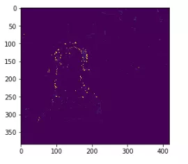
import cv2
import numpy as np
import matplotlib.pyplot as plt
def calc_backproject():
    sample = cv2.imread("./sample_img/sample.png")
    target = cv2.imread("./sample_img/target.png")
    roi_hsv = cv2.cvtColor(sample, cv2.COLOR_BGR2HSV)
    target_hsv = cv2.cvtColor(target, cv2.COLOR_BGR2HSV)
    cv2.imshow("sample", sample)
    cv2.imshow("target", target)
    roiHist = cv2.calcHist(roi_hsv, [0, 1], None,
                           [30, 30], [0, 180, 0, 256])
    cv2.normalize(roiHist, roiHist, 0, 255, cv2.NORM_MINMAX)
    dst = cv2.calcBackProject([target_hsv], [0, 1],
                              roiHist, [0, 180, 0, 256], 1)
    cv2.imshow("dst", dst)
    plt.imshow(dst)
calc_backproject()
cv2.waitKey(0)
cv2.destroyAllWindows()

模板匹配

理论

学习目标

• 查找图像中的指定对象
• cv2.matchTemplate(), cv2.minMaxLoc()

在一副图像中查找与模板图像最匹配（相似）的部分。对模板图像进行滑动匹配源图像

matchTemplate(image, templ, method[, result[, mask]]) -> result

• image: 待搜索图像， 8 位或者 32 位浮点型图像 大小： W×H
• templ: 搜索模板，需要和原图像有一样的数据类型，且大小不能超过原图像 大小： w×h
• method: 匹配方法
  • M_SQDIFF = 0, 平方差匹配 数值越小，有着越高的匹配结果
  • TM_SQDIFF_NORMED = 1, 归一化 平方差匹配 数值越小，有着越高的匹配结果
  • 以下方法，数值越小，匹配结果越好
  • TM_CCORR = 2, 相关匹配
  • TM_CCORR_NORMED = 3, 归一化相关匹配
  • TM_CCOEFF = 4, 系数匹配
  • TM_CCOEFF_NORMED = 5 归一化相关系数匹配
• result: 输出图像 大小 (W-w+1×H-h+1)
  模板匹配方法

简单法：平方差方法，速度快，但不是很精确
复杂法：相关系数法，计算量大，较精确
综合考虑选择运用哪种匹配方法

minMaxLoc(src[, mask]) -> minVal, maxVal, minLoc, maxLoc

• 函数功能：找到数组或者图像最小最大值及其位置
• src: 要查找的数组
• minVal, maxVal: 最小，最大值
• minLoc, maxLoc; 最小，最大值的位置

import numpy as np
img = np.array(np.arange(25)).reshape(5, 5)
print(img, cv2.minMaxLoc(img), sep='\n')

[[ 0  1  2  3  4]
 [ 5  6  7  8  9]
 [10 11 12 13 14]
 [15 16 17 18 19]
 [20 21 22 23 24]]
(0.0, 24.0, (0, 0), (4, 4))

eval() 用法说明

import cv2
methods = ['cv2.TM_CCOEFF', 'cv2.TM_CCOEFF_NORMED', 'cv2.TM_CCORR',
           'cv2.TM_CCORR_NORMED', 'cv2.TM_SQDIFF', 'cv2.TM_SQDIFF_NORMED']
for method in methods:
    print(eval(method)) # 可以判断 methods 里面的值在 OpenCV 中对应的值
    # 运行结果
'''
4
5
2
3
0
1
'''

例程

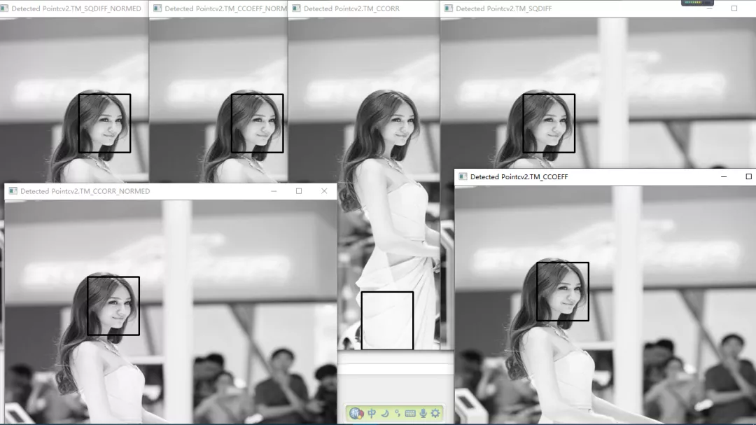
import cv2
import numpy as np
from matplotlib import pyplot as plt
img = cv2.imread('./sample_img/template (1).jpg', 0)
img = cv2.resize(img, (600, 600))
img2 = img.copy()
template = cv2.imread('./sample_img/template (2).jpg', 0)
w, h = template.shape[::-1]
# All the 6 methods for comparison in a list
methods = ['cv2.TM_CCOEFF', 'cv2.TM_CCOEFF_NORMED', 'cv2.TM_CCORR',
           'cv2.TM_CCORR_NORMED', 'cv2.TM_SQDIFF', 'cv2.TM_SQDIFF_NORMED']
for meth in methods:
    img = img2.copy()
    method = eval(meth) # 可以判断 methods 里面的值在 OpenCV 中对应的值
    # Apply template Matching
    res = cv2.matchTemplate(img, template, method)
    min_val, max_val, min_loc, max_loc = cv2.minMaxLoc(res)
    #print(res)
    # If the method is TM_SQDIFF or TM_SQDIFF_NORMED, take minimum
    if method in [cv2.TM_SQDIFF, cv2.TM_SQDIFF_NORMED]:
        top_left = min_loc
    else:
        top_left = max_loc
    bottom_right = (top_left[0] + w, top_left[1] + h)
    cv2.rectangle(img, top_left, bottom_right, (0, 0, 255), 2)
    #cv2.imshow('Matching Result'+str(meth), res)
    cv2.imshow('Detected Point'+str(meth), img)
cv2.waitKey(0)
cv2.destroyAllWindows()

cv2.TM_CCORR 方法的效果不是很好

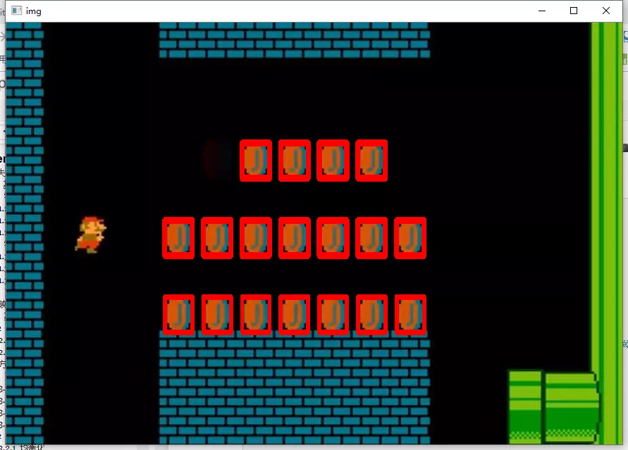
多目标匹配

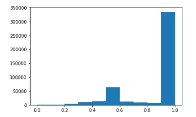
cv2.TM_CCOEFF_NORMED 方法

import cv2
import numpy as np
import time
t0 = time.time()
img = cv2.imread("./sample_img/mario.jpg")
template = img[170:220, 334:373, :]
img_gray = cv2.cvtColor(img, cv2.COLOR_BGR2GRAY)
template = cv2.cvtColor(template, cv2.COLOR_BGR2GRAY)
w, h = template.shape[::-1]
res = cv2.matchTemplate(img_gray, template, cv2.TM_CCOEFF_NORMED) # 用归一化的方法，阈值的设定比较方便
threshold = 0.8 # 表示模板和检测目标 80% 的匹配程度就认为是所要查找的目标
loc = np.where(res >= threshold)
for pt in zip(*loc[::-1]):
    cv2.rectangle(img, pt, (pt[0] + w, pt[1] + h), (0, 0, 255), 2)
print("time:", time.time()-t0)
cv2.imshow("img", img)
cv2.waitKey(0)
cv2.destroyAllWindows()

time: 0.07096028327941895

import matplotlib.pyplot as plt
plt.hist(res.ravel());

cv2.TM_SQDIFF_NORMED 方法

import cv2
import numpy as np
import time
t0 = time.time()
img = cv2.imread("./sample_img/mario.jpg")
template = img[170:220, 334:373, :]
img_gray = cv2.cvtColor(img, cv2.COLOR_BGR2GRAY)
template = cv2.cvtColor(template, cv2.COLOR_BGR2GRAY)
w, h = template.shape[::-1]
res = cv2.matchTemplate(img_gray, template, cv2.TM_SQDIFF_NORMED) # 在
threshold = 0.2 # 表示模板和检测目标 80% 的匹配程度就认为是所要查找的目标
loc = np.where(res <= threshold)
for pt in zip(*loc[::-1]):
    cv2.rectangle(img, pt, (pt[0] + w, pt[1] + h), (0, 0, 255), 2)
print("time:", time.time()-t0)
cv2.imshow("img", img)
cv2.waitKey(0)
cv2.destroyAllWindows()

time: 0.09594225883483887

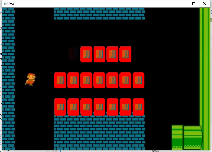
cv2.TM_CCORR_NORMED 方法

import cv2
import numpy as np
import time
t0 = time.time()
img = cv2.imread("./sample_img/mario.jpg")
template = img[170:220, 334:373, :]
img_gray = cv2.cvtColor(img, cv2.COLOR_BGR2GRAY)
template = cv2.cvtColor(template, cv2.COLOR_BGR2GRAY)
w, h = template.shape[::-1]
res = cv2.matchTemplate(img_gray, template, cv2.TM_CCORR_NORMED) # 在
threshold = 0.95 # 表示模板和检测目标 80% 的匹配程度就认为是所要查找的目标
loc = np.where(res >= threshold)
for pt in zip(*loc[::-1]):
    cv2.rectangle(img, pt, (pt[0] + w, pt[1] + h), (0, 0, 255), 2)
print("time:", time.time()-t0)
cv2.imshow("img", img)
cv2.waitKey(0)
cv2.destroyAllWindows()

time: 0.05097007751464844

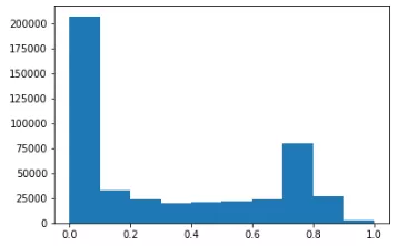
此方法把一个不是很明显的目标也检测出来，此方法的性能估计比较高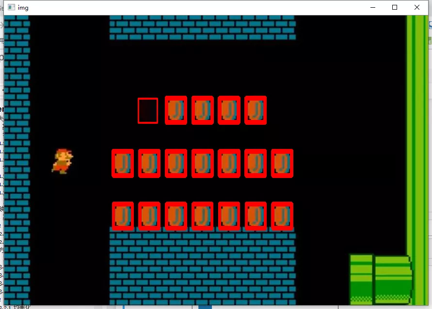

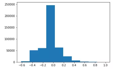
import matplotlib.pyplot as plt
plt.hist(res.ravel());

Tips

a = [1, 2, 3, 4]
a[::-1] # 反转
#结果  [4, 3, 2, 1]

Python zip 功能说明

a = [1, 2, 3]
b = [4, 5, 6]
c = [4, 5, 6, 7, 8]
zipped = zip(a, b)     # 打包为元组的列表
[k for k in zip(*zipped)]          # 与 zip 相反，*zipped 可理解为解压，返回二维矩阵式
# 结果 [(1, 2, 3), (4, 5, 6)]