一、随机森林
二、用随机森林回归填补缺失值
- 以波士顿数据集为例，导入完整的数据集并探索
- 为完整数据集放入缺失值
1. 用0填充缺失值
2. 用均值填充缺失值
- 3. 用随机森林回归填补缺失值
- 4. 评估
三、随机森林在乳腺癌数据上的调参

一、随机森林

集成算法

集成学习（ensemble learning）不是一个单独的机器学习算法，而是通过在数据上构建多个模型，集成所有模型的建模结果。基本上所有机器学习领域都可以看到集成学习的身影，它可以用来做市场营销模拟的建模，统计客户来源，保留和流失，也可用来预测疾病的风险和病患者的易感性。在现在的各种算法竞赛中，随机森林，梯度提升树（GBDT），Xgboost等集成算法也随处可见。

集成算法的目标：集成算法会考虑多个评估器的建模结果，汇总之后得到一个综合的结果，以此来获取比单个模型更好的回归或分类表现。

多个模型集成成为的模型叫做 集成评估器 （ensemble estimator），组成集成评估器的每个模型都叫做 基评估器 （base estimator）。通常来说，有三类集成算法：装袋法（Bagging），提升法（Boosting）和stacking。

装袋法的核心思想是构建多个相互独立的评估器，然后对其预测进行平均或多数表决原则来决定集成评估器的结果。装袋法的代表模型就是随机森林。提升法中，基评估器是相关的，是按顺序一一构建的。其核心思想是结合弱评估器的力量一次次对难以评估的样本进行预测，从而构成一个强评估器。提升法的代表模型有Adaboost和梯度提升树。

随机森林分类器RandomForestClassifier

随机森林是非常具有代表性的Bagging集成算法，所有基评估器都是决策树，分类树组成的森林就叫做随机森林分类器，回归树所集成的森林就叫做随机森林回归器。

控制基评估器的参数

参数	含义
criterion	不纯度的衡量指标，有基尼系数和信息熵两种选择
max_depth	树的最大深度，超过最大深度的树枝都会被剪掉
min_samples_leaf	一个节点在分枝后的每个子节点都必须包含至少min_samples_leaf个训练样本，否则分枝就不会发生
min_samples_split	一个节点必须要包含至少min_samples_split个训练样本，这个节点才允许被分枝，否则分枝就不会发生
max_features max_features	限制分枝时考虑的特征个数，超过限制个数的特征都会被舍弃，

默认值为总特征个数开平方取整 | | min_impurity_decrease | 限制信息增益的大小，信息增益小于设定数值的分枝不会发生 |

sklearn建模基本流程

分测试集和训练集

【注意】在skleran中，特征和标签需要分开导入 先X后Y，先train后test：Xtrain, Xtest, Ytrain, Ytest

实例化
把训练集带入实例化后的模型训练，

使用接口fit
使用其他接口将测试集导入训练好的模型

获取结果：score（score接口）/Y_test（predict接口）
探索模型的稳定性
1. 交叉验证
  1. 实例化
  2. 以完整的特征集和标签集为参数，交叉验证自动划分训练集与测试集
  3. 绘图

学习曲线
oobscore属性

import numpy as np
import pandas as pd
from sklearn.tree import DecisionTreeClassifier
from sklearn.ensemble import RandomForestClassifier
from sklearn.datasets import load_wine
from sklearn.model_selection import train_test_split
from sklearn.model_selection import cross_val_score
# 交叉验证会自动分好训练集和测试集，不需要train_test_split
from scipy.special import comb
import matplotlib.pyplot as plt
%matplotlib inline

wine = load_wine()

Xtrain, Xtest, Ytrain, Ytest = train_test_split(wine.data, wine.target, test_size = 0.3)

clf = DecisionTreeClassifier(random_state = 0)
rfc = RandomForestClassifier(random_state = 0)
clf = clf.fit(Xtrain, Ytrain)
rfc = rfc.fit(Xtrain, Ytrain)
score_c = clf.score(Xtest, Ytest)
score_r = rfc.score(Xtest, Ytest)
print('Single Tree:{}'.format(score_c), '\nRandom Forest:{}'.format(score_r))
print()

Single Tree:0.8703703703703703 
Random Forest:0.9814814814814815
C:\anaconda\lib\site-packages\sklearn\ensemble\forest.py:245: FutureWarning: The default value of n_estimators will change from 10 in version 0.20 to 100 in 0.22.
  "10 in version 0.20 to 100 in 0.22.", FutureWarning)

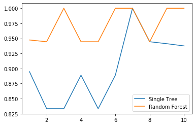
交叉验证：画出随机森林与决策树在一组交叉验证下的效果对比

clf = DecisionTreeClassifier()
rfc = RandomForestClassifier(n_estimators = 25)
score_c = cross_val_score(clf, wine.data, wine.target, cv = 10)
score_r = cross_val_score(rfc, wine.data, wine.target, cv = 10)
plt.plot(range(1, 11), score_c, label = 'Single Tree') # 一个plot中可以画多条线，但只能有一个标签
plt.plot(range(1, 11), score_r, label = 'Random Forest')
plt.legend()

<matplotlib.legend.Legend at 0x1e8d82f8cf8>

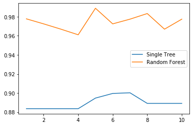
画出随机森林与决策树在十组交叉验证下的效果对比

score_c = []
score_r = []
for i in range(10):
    clf = DecisionTreeClassifier()
    rfc = RandomForestClassifier(n_estimators = 25)
    score_c.append(cross_val_score(clf, wine.data, wine.target, cv = 10).mean())
    score_r.append(cross_val_score(rfc, wine.data, wine.target, cv = 10).mean())
plt.plot(range(1, 11), score_c, label = 'Single Tree')
plt.plot(range(1, 11), score_r, label = 'Random Forest')
plt.legend()

<matplotlib.legend.Legend at 0x1e8da38fe48>

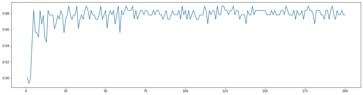
n_estimators的学习曲线

superpa = []
for i in range(200):
    rfc = RandomForestClassifier(n_estimators=i+1,n_jobs=-1)
    rfc_s = cross_val_score(rfc,wine.data,wine.target,cv=10).mean()
    superpa.append(rfc_s)
print(max(superpa),superpa.index(max(superpa))+1)#打印出：最高精确度取值，max(superpa))+1指的是森林数目的数量n_estimators
plt.figure(figsize=[20,5])
plt.plot(range(1,201),superpa)

0.9888888888888889 27
[<matplotlib.lines.Line2D at 0x1e8d95736d8>]

重要属性：estimators_

np.array([comb(25, i) * (0.2 ** i) * (0.8 ** (25 - i)) for i in range(13, 26)]).sum()

0.00036904803455582827

rfc = RandomForestClassifier(n_estimators = 25, random_state = 2)
rfc = rfc.fit(Xtrain, Ytrain)

rfc.estimators_[:2]

[DecisionTreeClassifier(class_weight=None, criterion='gini', max_depth=None,
                        max_features='auto', max_leaf_nodes=None,
                        min_impurity_decrease=0.0, min_impurity_split=None,
                        min_samples_leaf=1, min_samples_split=2,
                        min_weight_fraction_leaf=0.0, presort=False,
                        random_state=1462290116, splitter='best'),
 DecisionTreeClassifier(class_weight=None, criterion='gini', max_depth=None,
                        max_features='auto', max_leaf_nodes=None,
                        min_impurity_decrease=0.0, min_impurity_split=None,
                        min_samples_leaf=1, min_samples_split=2,
                        min_weight_fraction_leaf=0.0, presort=False,
                        random_state=2007616322, splitter='best')]

for i in range(len(rfc.estimators_)):
    print(rfc.estimators_[i].random_state)

oobscore属性

rfc = RandomForestClassifier(n_estimators = 25, oob_score = True)
rfc.fit(wine.data, wine.target)
rfc.oob_score_

0.9719101123595506

其他重要属性和接口

rfc = RandomForestClassifier(n_estimators = 25, oob_score = True)
rfc.fit(Xtrain, Ytrain)

RandomForestClassifier(bootstrap=True, class_weight=None, criterion='gini',
                       max_depth=None, max_features='auto', max_leaf_nodes=None,
                       min_impurity_decrease=0.0, min_impurity_split=None,
                       min_samples_leaf=1, min_samples_split=2,
                       min_weight_fraction_leaf=0.0, n_estimators=25,
                       n_jobs=None, oob_score=True, random_state=None,
                       verbose=0, warm_start=False)

rfc.score(Xtest, Ytest)

0.9814814814814815

rfc.feature_importances_

array([0.04545681, 0.05468689, 0.01279688, 0.03417742, 0.02951136,
       0.05256852, 0.1602701 , 0.00956776, 0.00705849, 0.18598547,
       0.10212229, 0.04885997, 0.25693803])

[*zip(wine.feature_names, rfc.feature_importances_)]

[('alcohol', 0.04545681330313256),
 ('malic_acid', 0.05468689429182469),
 ('ash', 0.01279688364085699),
 ('alcalinity_of_ash', 0.03417741743145594),
 ('magnesium', 0.029511363752189344),
 ('total_phenols', 0.052568517086408285),
 ('flavanoids', 0.16027009795568858),
 ('nonflavanoid_phenols', 0.009567755401484716),
 ('proanthocyanins', 0.007058492408035047),
 ('color_intensity', 0.18598547273378016),
 ('hue', 0.10212229034493969),
 ('od280/od315_of_diluted_wines', 0.0488599676410731),
 ('proline', 0.25693803400913084)]

rfc.apply(Xtest)

array([[ 4,  9, 11, ..., 13,  8,  5],
       [19, 10,  8, ..., 10, 12, 11],
       [17,  4,  3, ...,  2,  9,  5],
       ...,
       [ 4,  9, 13, ..., 16,  8, 17],
       [17,  2,  3, ...,  2,  3,  5],
       [21, 10, 15, ..., 22, 18, 22]], dtype=int64)

rfc.predict(Xtest)

array([2, 1, 1, 1, 1, 2, 1, 0, 2, 1, 1, 1, 2, 2, 1, 0, 0, 0, 0, 1, 1, 1,
       1, 1, 0, 1, 0, 2, 2, 2, 1, 2, 2, 1, 2, 1, 1, 2, 0, 2, 0, 2, 2, 0,
       1, 0, 2, 0, 1, 1, 2, 2, 1, 0])

Ytest

array([2, 1, 1, 1, 1, 2, 1, 0, 2, 1, 1, 1, 2, 1, 1, 0, 0, 0, 0, 1, 1, 1,
       1, 1, 0, 1, 0, 2, 2, 2, 1, 2, 2, 1, 2, 1, 1, 2, 0, 2, 0, 2, 2, 0,
       1, 0, 2, 0, 1, 1, 2, 2, 1, 0])

rfc.predict_proba(Xtest)[:10]

array([[0.  , 0.12, 0.88],
       [0.24, 0.68, 0.08],
       [0.  , 1.  , 0.  ],
       [0.  , 1.  , 0.  ],
       [0.  , 1.  , 0.  ],
       [0.  , 0.04, 0.96],
       [0.04, 0.96, 0.  ],
       [1.  , 0.  , 0.  ],
       [0.08, 0.04, 0.88],
       [0.32, 0.48, 0.2 ]])

Bagging的另一个必要条件

np.array([comb(25, i) * (0.5 ** i) * (0.5 ** (25 - i)) for i in range(13, 26)]).sum()

0.5

y = []
for epsilon in np.linspace(0, 1, 20):
    E = np.array([comb(25, i) * (epsilon ** i) * ((1 - epsilon) ** (25 - i)) for i in range(13, 26)]).sum()
    y.append(E)
plt.plot(np.linspace(0, 1, 20), y, '-o', label = 'when estimators are different')
plt.plot(np.linspace(0, 1, 20), np.linspace(0, 1, 20), '--', label = 'if all estimators are same')
plt.xlabel("individual estimator's error")
plt.ylabel("RandomForest's error")
plt.legend()

<matplotlib.legend.Legend at 0x1e8da435cf8>

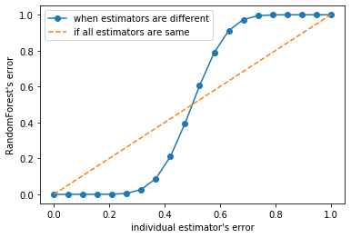
基分类器的准确率至少要超过50%，随机森林算法才能有好的效果
所以在使用随机森林之前，一定要检查用来组成随机森林的分类树是否都有至少50%以上的准确率

随机森林回归器RandomForestRegressor

from sklearn.datasets import load_boston
from sklearn.ensemble import RandomForestRegressor

load_boston = load_boston()

rfr1 = RandomForestRegressor(n_estimators = 100, random_state = 0)
Xtrain, Xtest, Ytrain, Ytest = train_test_split(load_boston.data, load_boston.target, test_size = 0.3)
rfr1 = rfr1.fit(Xtrain, Ytrain)
score = cross_val_score(rfr1, load_boston.data, load_boston.target, cv = 10, scoring = 'neg_mean_squared_error')

score

array([-10.72900447,  -5.36049859,  -4.74614178, -20.84946337,
       -12.23497347, -17.99274635,  -6.8952756 , -93.78884428,
       -29.80411702, -15.25776814])

rfr2 = RandomForestRegressor(n_estimators = 100, random_state = 0)
score = cross_val_score(rfr2, load_boston.data, load_boston.target, cv = 10, scoring = 'neg_mean_squared_error')

score

array([-10.72900447,  -5.36049859,  -4.74614178, -20.84946337,
       -12.23497347, -17.99274635,  -6.8952756 , -93.78884428,
       -29.80411702, -15.25776814])

sklearn中的模型评分指标

from sklearn.metrics import SCORERS

sorted(SCORERS.keys())[:10]

['accuracy',
 'adjusted_mutual_info_score',
 'adjusted_rand_score',
 'average_precision',
 'balanced_accuracy',
 'brier_score_loss',
 'completeness_score',
 'explained_variance',
 'f1',
 'f1_macro']

二、用随机森林回归填补缺失值

用0填充
用均值填充
随机森林回归填补
几种填补方法与原始数据集对比

以波士顿数据集为例，导入完整的数据集并探索

from sklearn.impute import SimpleImputer # 填补缺失值的类

dataset = load_boston
dataset.data.shape

(506, 13)

# 共有506*13=6578个数据
x_full, y_full = dataset.data, dataset.target
n_samples = x_full.shape[0]
n_features = x_full.shape[1]

为完整数据集放入缺失值

是在特征中放入空值，而不是在标签中放入，标签不能空，否则就成了无监督学习

rng = np.random.RandomState(0) # 随机数种子固定随机模式
# 确定我们希望放入的缺失值的比例，在此我们假设50%，那就总共有3289个数据缺失
missing_rate = 0.5
n_missing_samples = int(np.floor(n_samples * n_features * missing_rate)) 
# 1. 向下取整，返回.0格式的浮点数
# 2. 将浮点数转换为整数
n_missing_samples

# 所有数据要随机遍布在数据集的各行各列当中，而一个缺失的数据会需要一个行索引和一个列索引
# 创造放置索引的数组，包含3289个分布在0~506中间的行索引，和3289个分布在0~13之间的列索引
# 利用索引来为数据中的任意3289个位置赋空值
missing_features = rng.randint(0, n_features, n_missing_samples)
missing_samples = rng.randint(0, n_samples, n_missing_samples) 
# 如果我们需要的数据量小于我们的样本量506，那我们可以采用np.random.choice来抽样，choice会随机抽取不重复的随机数
# np.random.choice可以让数据更加分散，确保数据不会集中在一些行中
# 这里我们不采用np.random.choice,因为我们现在采样了3289个数据，远远超过我们的样本量506，使用np.random.choice会报错

x_missing = x_full.copy()
y_missing = y_full.copy()
x_missing[missing_samples, missing_features] = None

x_missing[:5]

array([[       nan, 1.8000e+01,        nan,        nan, 5.3800e-01,
               nan, 6.5200e+01, 4.0900e+00, 1.0000e+00, 2.9600e+02,
               nan,        nan, 4.9800e+00],
       [2.7310e-02, 0.0000e+00,        nan, 0.0000e+00, 4.6900e-01,
               nan, 7.8900e+01, 4.9671e+00, 2.0000e+00,        nan,
               nan, 3.9690e+02, 9.1400e+00],
       [2.7290e-02,        nan, 7.0700e+00, 0.0000e+00,        nan,
        7.1850e+00, 6.1100e+01,        nan, 2.0000e+00, 2.4200e+02,
               nan,        nan,        nan],
       [       nan,        nan,        nan, 0.0000e+00, 4.5800e-01,
               nan, 4.5800e+01,        nan,        nan, 2.2200e+02,
        1.8700e+01,        nan,        nan],
       [       nan, 0.0000e+00, 2.1800e+00, 0.0000e+00,        nan,
        7.1470e+00,        nan,        nan,        nan,        nan,
        1.8700e+01,        nan, 5.3300e+00]])

x_missing = pd.DataFrame(x_missing)

x_missing.head()

	0	1	2	3	4	5	6	7	8	9	10	11	12
0	NaN	18.0	NaN	NaN	0.538	NaN	65.2	4.0900	1.0	296.0	NaN	NaN	4.98
1	0.02731	0.0	NaN	0.0	0.469	NaN	78.9	4.9671	2.0	NaN	NaN	396.9	9.14
2	0.02729	NaN	7.07	0.0	NaN	7.185	61.1	NaN	2.0	242.0	NaN	NaN	NaN
3	NaN	NaN	NaN	0.0	0.458	NaN	45.8	NaN	NaN	222.0	18.7	NaN	NaN
4	NaN	0.0	2.18	0.0	NaN	7.147	NaN	NaN	NaN	NaN	18.7	NaN	5.33

1. 用0填充缺失值

x_missing = x_full.copy()
y_missing = y_full.copy()
x_missing[missing_samples, missing_features] = None
x_missing = pd.DataFrame(x_missing)
# 实例化
imp_zero = SimpleImputer(missing_values = np.nan, strategy = 'constant', fill_value = 0)
# 接口fit_transform：fit（训练） + predict（导出）
x_missing_zero = imp_zero.fit_transform(x_missing)
x_missing_zero

array([[0.0000e+00, 1.8000e+01, 0.0000e+00, ..., 0.0000e+00, 0.0000e+00,
        4.9800e+00],
       [2.7310e-02, 0.0000e+00, 0.0000e+00, ..., 0.0000e+00, 3.9690e+02,
        9.1400e+00],
       [2.7290e-02, 0.0000e+00, 7.0700e+00, ..., 0.0000e+00, 0.0000e+00,
        0.0000e+00],
       ...,
       [0.0000e+00, 0.0000e+00, 1.1930e+01, ..., 2.1000e+01, 0.0000e+00,
        5.6400e+00],
       [1.0959e-01, 0.0000e+00, 1.1930e+01, ..., 2.1000e+01, 3.9345e+02,
        6.4800e+00],
       [4.7410e-02, 0.0000e+00, 1.1930e+01, ..., 0.0000e+00, 3.9690e+02,
        7.8800e+00]])

pd.DataFrame(x_missing_zero).isnull().sum()

0     0
1     0
2     0
3     0
4     0
5     0
6     0
7     0
8     0
9     0
10    0
11    0
12    0
dtype: int64

2. 用均值填充缺失值

x_missing = x_full.copy()
y_missing = y_full.copy()
x_missing[missing_samples, missing_features] = None
x_missing = pd.DataFrame(x_missing)
# 实例化
imp_mean = SimpleImputer(missing_values = np.nan, strategy = 'mean')
# 接口fit_transform：fit（训练） + predict（导出）
x_missing_mean = imp_mean.fit_transform(x_missing)
x_missing_mean

array([[3.62757895e+00, 1.80000000e+01, 1.11634641e+01, ...,
        1.85211921e+01, 3.52741952e+02, 4.98000000e+00],
       [2.73100000e-02, 0.00000000e+00, 1.11634641e+01, ...,
        1.85211921e+01, 3.96900000e+02, 9.14000000e+00],
       [2.72900000e-02, 1.07229508e+01, 7.07000000e+00, ...,
        1.85211921e+01, 3.52741952e+02, 1.29917666e+01],
       ...,
       [3.62757895e+00, 1.07229508e+01, 1.19300000e+01, ...,
        2.10000000e+01, 3.52741952e+02, 5.64000000e+00],
       [1.09590000e-01, 0.00000000e+00, 1.19300000e+01, ...,
        2.10000000e+01, 3.93450000e+02, 6.48000000e+00],
       [4.74100000e-02, 0.00000000e+00, 1.19300000e+01, ...,
        1.85211921e+01, 3.96900000e+02, 7.88000000e+00]])

pd.DataFrame(x_missing_mean).isnull().sum()

0     0
1     0
2     0
3     0
4     0
5     0
6     0
7     0
8     0
9     0
10    0
11    0
12    0
dtype: int64

3. 用随机森林回归填补缺失值

x_missing_reg = x_missing.copy()
# 找出数据集中，缺失值从小到大排列的特征们的顺序
sortindex = np.argsort(x_missing_reg.isnull().sum()).values
# argsort返回的是，特征按缺失值数量从小到大排序的顺序，及原来对应的索引

for i in sortindex:
    # 构建新特征矩阵和新标签
    df = x_missing_reg
    fillc = df.iloc[:, i]
    df = pd.concat([df.iloc[:, df.columns != i], pd.DataFrame(y_full)], axis = 1)
    # 用0填充新矩阵的缺失值
    imp_zero = SimpleImputer(missing_values = np.nan, strategy = 'constant', fill_value = 0)
    df_zero = imp_zero.fit_transform(df)
    # 分开训练集和测试集
    Ytrain = fillc[fillc.notnull()]
    Ytest = fillc[fillc.isnull()]
    Xtrain = df_zero[Ytrain.index, :]
    Xtest = df_zero[Ytest.index, :]
    # 用回归森林回归填补缺失值
    rfr = RandomForestRegressor(n_estimators = 100)
    rfr.fit(Xtrain, Ytrain)
    x_missing_reg.loc[x_missing_reg.iloc[:, i].isnull(), i] = rfr.predict(Xtest)

x_missing_reg.head()

	0	1	2	3	4	5	6	7	8	9	10	11	12
0	0.280164	18.00	6.6453	0.14	0.538000	6.59824	65.200	4.090000	1.00	296.00	18.213	389.5860	4.9800
1	0.027310	0.00	6.1291	0.00	0.469000	6.18508	78.900	4.967100	2.00	305.16	18.135	396.9000	9.1400
2	0.027290	11.38	7.0700	0.00	0.462928	7.18500	61.100	4.311964	2.00	242.00	17.824	388.4907	5.3172
3	0.096453	16.69	2.8925	0.00	0.458000	6.92689	45.800	4.784298	3.70	222.00	18.700	393.6865	5.9258
4	0.115528	0.00	2.1800	0.00	0.467328	7.14700	59.009	4.834263	3.74	247.62	18.700	392.3946	5.3300

4. 评估

X = [x_missing_zero, x_missing_mean, x_missing_reg, x_full]
mse = []
for x in X:
    estimators = RandomForestRegressor(random_state = 0, n_estimators = 100)
    score = cross_val_score(estimators, x, y_full, scoring = 'neg_mean_squared_error', cv = 5).mean()
    mse.append(score * -1)

[*zip(['x_missing_zero', 'x_missing_mean', 'x_missing_reg', 'x_full'], mse)]

[('x_missing_zero', 49.50657028893417),
 ('x_missing_mean', 40.84405476955929),
 ('x_missing_reg', 21.372347360920205),
 ('x_full', 21.62860460743544)]

x_labels = ['Zero Imputation', 'Mean Imputation', 'Regressor Imputation', 'Full Data']
colors = ['r', 'g', 'b', 'orange']
plt.figure(figsize = (12, 6)) # 创建画布
ax = plt.subplot(111) # 创建子图
for i in np.arange(len(mse)):
    ax.barh(i, mse[i], color = colors[i], alpha = .6, align = 'center')
ax.set_title('Imputation Techniques with Boston Data')
ax.set_xlim(left = np.min(mse) * 0.9, right = np.max(mse) * 1.1)
ax.set_yticks(np.arange(len(mse)))
ax.set_xlabel('MSE')
ax.invert_yaxis() # y轴刻度倒过来
ax.set_yticklabels(x_labels)

[Text(0, 0, 'Zero Imputation'),
 Text(0, 0, 'Mean Imputation'),
 Text(0, 0, 'Regressor Imputation'),
 Text(0, 0, 'Full Data')]

回归的数据集比原始数据集的表现还要好，有过拟合的风险

三、随机森林在乳腺癌数据上的调参

from sklearn.datasets import load_breast_cancer
from sklearn.model_selection import GridSearchCV

data = load_breast_cancer()

data.data.shape

(569, 30)

np.unique(data.target)

array([0, 1])

rfc = RandomForestClassifier(n_estimators = 100, random_state = 90) # 实例化
score_pre = cross_val_score(rfc, data.data, data.target, cv = 10, scoring = 'accuracy').mean()
score_pre

0.9666925935528475

1. n_estimators

score = []
for i in range(0, 200, 10):
    rfc = RandomForestClassifier(n_estimators = i + 1, random_state = 90)
    score_ = cross_val_score(rfc, data.data, data.target, cv = 10).mean()
    score.append(score_)
plt.figure(figsize = (20, 5))
plt.plot(range(1, 201, 10), score)

[<matplotlib.lines.Line2D at 0x1e8e26bd9e8>]

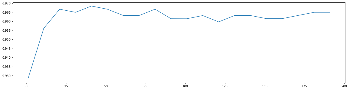
print(max(score), score.index(max(score)) * 10 + 1)

0.9684480598046841 41

score = []
for i in range(35, 45):
    rfc = RandomForestClassifier(n_estimators = i, n_jobs = -1, random_state = 90)
    score_pre = cross_val_score(rfc, data.data, data.target, cv = 10).mean()
    score.append(score_pre)
plt.figure(figsize = (20, 5))
plt.plot(range(35, 45), score)

[<matplotlib.lines.Line2D at 0x1e8e09d7fd0>]

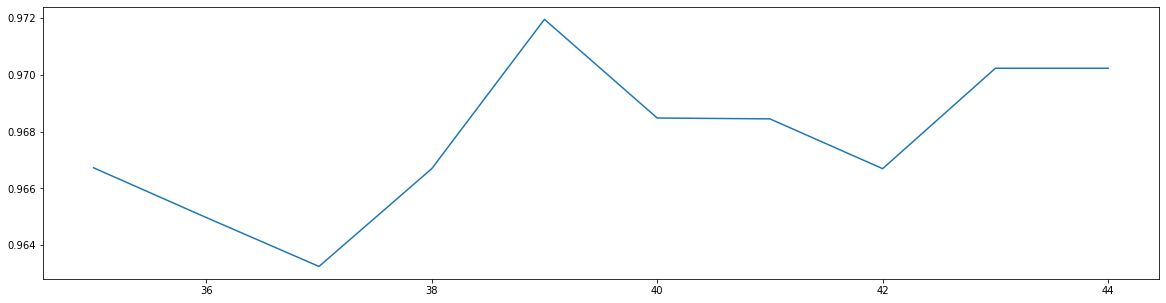
print(max(score), [*range(35, 45)][score.index(max(score))])

0.9719568317345088 39

2. max_depth

param_grid = {'max_depth':np.arange(1, 20, 1)}
rfc = RandomForestClassifier(n_estimators = 39, random_state = 90)
GS = GridSearchCV(rfc, param_grid, cv = 10)
GS.fit(data.data, data.target)

C:\anaconda\lib\site-packages\sklearn\model_selection\_search.py:813: DeprecationWarning: The default of the `iid` parameter will change from True to False in version 0.22 and will be removed in 0.24. This will change numeric results when test-set sizes are unequal.
  DeprecationWarning)
GridSearchCV(cv=10, error_score='raise-deprecating',
             estimator=RandomForestClassifier(bootstrap=True, class_weight=None,
                                              criterion='gini', max_depth=None,
                                              max_features='auto',
                                              max_leaf_nodes=None,
                                              min_impurity_decrease=0.0,
                                              min_impurity_split=None,
                                              min_samples_leaf=1,
                                              min_samples_split=2,
                                              min_weight_fraction_leaf=0.0,
                                              n_estimators=39, n_jobs=None,
                                              oob_score=False, random_state=90,
                                              verbose=0, warm_start=False),
             iid='warn', n_jobs=None,
             param_grid={'max_depth': array([ 1,  2,  3,  4,  5,  6,  7,  8,  9, 10, 11, 12, 13, 14, 15, 16, 17,
       18, 19])},
             pre_dispatch='2*n_jobs', refit=True, return_train_score=False,
             scoring=None, verbose=0)

GS.best_params_

{'max_depth': 11}

GS.best_score_

0.9718804920913884

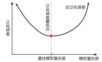
准确率不升反降，泛化误差上升的同时，可能是复杂度不够
minsamples_leaf 和 min_samples_split 是剪枝参数，不适合再调整

3. max_features

param_grid = {'max_features':np.arange(5, 30, 1)}
rfc = RandomForestClassifier(n_estimators = 39, random_state = 90)
GS = GridSearchCV(rfc, param_grid, cv = 10)
GS.fit(data.data, data.target)

C:\anaconda\lib\site-packages\sklearn\model_selection\_search.py:813: DeprecationWarning: The default of the `iid` parameter will change from True to False in version 0.22 and will be removed in 0.24. This will change numeric results when test-set sizes are unequal.
  DeprecationWarning)
GridSearchCV(cv=10, error_score='raise-deprecating',
             estimator=RandomForestClassifier(bootstrap=True, class_weight=None,
                                              criterion='gini', max_depth=None,
                                              max_features='auto',
                                              max_leaf_nodes=None,
                                              min_impurity_decrease=0.0,
                                              min_impurity_split=None,
                                              min_samples_leaf=1,
                                              min_samples_split=2,
                                              min_weight_fraction_leaf=0.0,
                                              n_estimators=39, n_jobs=None,
                                              oob_score=False, random_state=90,
                                              verbose=0, warm_start=False),
             iid='warn', n_jobs=None,
             param_grid={'max_features': array([ 5,  6,  7,  8,  9, 10, 11, 12, 13, 14, 15, 16, 17, 18, 19, 20, 21,
       22, 23, 24, 25, 26, 27, 28, 29])},
             pre_dispatch='2*n_jobs', refit=True, return_train_score=False,
             scoring=None, verbose=0)

GS.best_params_

{'max_features': 5}

GS.best_score_

0.9718804920913884

网格搜索给出的是设定的max_features的最小值，max_features升高也没有效果，可见模型目前可能已经处于泛化误差的最低点
随机森林分类的决策上界

4. min_samples_leaf

param_grid = {'min_samples_leaf':np.arange(1, 1 + 10, 1)}
rfc = RandomForestClassifier(n_estimators = 39, random_state = 90)
GS = GridSearchCV(rfc, param_grid, cv = 10)
GS.fit(data.data, data.target)

C:\anaconda\lib\site-packages\sklearn\model_selection\_search.py:813: DeprecationWarning: The default of the `iid` parameter will change from True to False in version 0.22 and will be removed in 0.24. This will change numeric results when test-set sizes are unequal.
  DeprecationWarning)
GridSearchCV(cv=10, error_score='raise-deprecating',
             estimator=RandomForestClassifier(bootstrap=True, class_weight=None,
                                              criterion='gini', max_depth=None,
                                              max_features='auto',
                                              max_leaf_nodes=None,
                                              min_impurity_decrease=0.0,
                                              min_impurity_split=None,
                                              min_samples_leaf=1,
                                              min_samples_split=2,
                                              min_weight_fraction_leaf=0.0,
                                              n_estimators=39, n_jobs=None,
                                              oob_score=False, random_state=90,
                                              verbose=0, warm_start=False),
             iid='warn', n_jobs=None,
             param_grid={'min_samples_leaf': array([ 1,  2,  3,  4,  5,  6,  7,  8,  9, 10])},
             pre_dispatch='2*n_jobs', refit=True, return_train_score=False,
             scoring=None, verbose=0)

GS.best_params_

{'min_samples_leaf': 1}

GS.best_score_

0.9718804920913884

5. min_samples_split

param_grid = {'min_samples_split':np.arange(2, 2 + 20, 1)}
rfc = RandomForestClassifier(n_estimators = 39, random_state = 90)
GS = GridSearchCV(rfc, param_grid, cv = 10)
GS.fit(data.data, data.target)

C:\anaconda\lib\site-packages\sklearn\model_selection\_search.py:813: DeprecationWarning: The default of the `iid` parameter will change from True to False in version 0.22 and will be removed in 0.24. This will change numeric results when test-set sizes are unequal.
  DeprecationWarning)
GridSearchCV(cv=10, error_score='raise-deprecating',
             estimator=RandomForestClassifier(bootstrap=True, class_weight=None,
                                              criterion='gini', max_depth=None,
                                              max_features='auto',
                                              max_leaf_nodes=None,
                                              min_impurity_decrease=0.0,
                                              min_impurity_split=None,
                                              min_samples_leaf=1,
                                              min_samples_split=2,
                                              min_weight_fraction_leaf=0.0,
                                              n_estimators=39, n_jobs=None,
                                              oob_score=False, random_state=90,
                                              verbose=0, warm_start=False),
             iid='warn', n_jobs=None,
             param_grid={'min_samples_split': array([ 2,  3,  4,  5,  6,  7,  8,  9, 10, 11, 12, 13, 14, 15, 16, 17, 18,
       19, 20, 21])},
             pre_dispatch='2*n_jobs', refit=True, return_train_score=False,
             scoring=None, verbose=0)

GS.best_params_

{'min_samples_split': 2}

GS.best_score_

0.9718804920913884

6. criterion

rfc = RandomForestClassifier(criterion = 'entropy', n_estimators = 39, random_state = 90)
score = cross_val_score(rfc, data.data, data.target, cv = 10).mean()
score

0.9649997839426151

rfc = RandomForestClassifier(criterion = 'gini', n_estimators = 39, random_state = 90)
score = cross_val_score(rfc, data.data, data.target, cv = 10).mean()
score

0.9719568317345088

数据分析_学习笔记

随机森林与医疗数据集调参

一、随机森林

集成算法

随机森林分类器RandomForestClassifier

控制基评估器的参数

sklearn建模基本流程

交叉验证：画出随机森林与决策树在一组交叉验证下的效果对比

画出随机森林与决策树在十组交叉验证下的效果对比

n_estimators的学习曲线

重要属性：estimators_

oobscore属性

其他重要属性和接口

Bagging的另一个必要条件

随机森林回归器RandomForestRegressor

sklearn中的模型评分指标

二、用随机森林回归填补缺失值

以波士顿数据集为例，导入完整的数据集并探索

为完整数据集放入缺失值

1. 用0填充缺失值

2. 用均值填充缺失值

3. 用随机森林回归填补缺失值

4. 评估

三、随机森林在乳腺癌数据上的调参

1. n_estimators

2. max_depth

3. max_features

4. min_samples_leaf

5. min_samples_split

6. criterion

随机森林与医疗数据集调参

一、 随机森林

集成算法

随机森林分类器RandomForestClassifier

控制基评估器的参数

sklearn建模基本流程

交叉验证：画出随机森林与决策树在一组交叉验证下的效果对比

画出随机森林与决策树在十组交叉验证下的效果对比

n_estimators的学习曲线

重要属性：estimators_

oobscore属性

其他重要属性和接口

Bagging的另一个必要条件

随机森林回归器RandomForestRegressor

sklearn中的模型评分指标

二、 用随机森林回归填补缺失值

以波士顿数据集为例，导入完整的数据集并探索

为完整数据集放入缺失值

1. 用0填充缺失值

2. 用均值填充缺失值

3. 用随机森林回归填补缺失值

4. 评估

三、 随机森林在乳腺癌数据上的调参

1. n_estimators

2. max_depth

3. max_features

4. min_samples_leaf

5. min_samples_split

6. criterion

一、随机森林

二、用随机森林回归填补缺失值

三、随机森林在乳腺癌数据上的调参